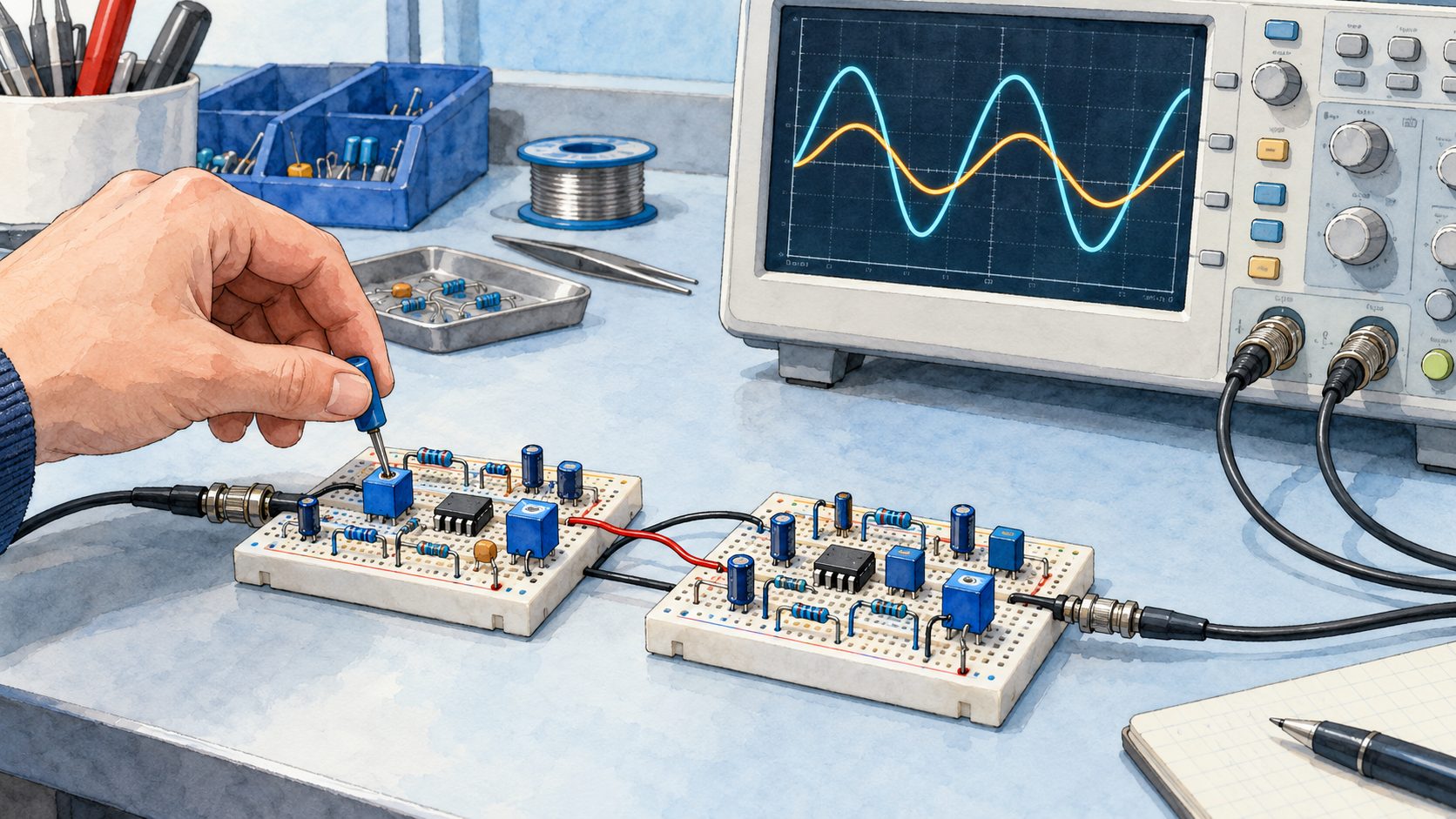
Take the Sallen–Key section from the previous part, tuned to 1\ \text{kHz} with a quality factor Q (the measure of its resonance) of 0.707. It attenuates by 3\ \text{dB} at its cutoff frequency—that is its definition. Put two of them in a row: the slope doubles, as expected, but at 1\ \text{kHz} the attenuation is now 6\ \text{dB}. The -3\ \text{dB} point has slipped to 800\ \text{Hz}, and your fourth-order filter has a narrower passband than either of the two sections it is made of.
The mistake is not in the wiring. It lies in the idea that a fourth-order filter is built by copying a second-order filter twice—and correcting it means going back to the polynomials that Butterworth, Bessel, Chebyshev and Cauer each proposed to answer the same question: what shape should the knee have?
In Part One, a passive RC section gave us a slope of -6\ \text{dB} per octave and nothing more. In Part Two, an operational amplifier gave us the quality factor Q, and with it control over the shape of the knee on one section. This third part answers the question that comes next, the one every serious specification asks: how to stack these sections to obtain the response we want, and not the response that stacking produces by accident.
Two correct filters, placed end to end, make a wrong filter
The number quoted in the introduction does not depend on the chosen frequency. The attenuations of two stages in series add up in decibels: at the common cutoff frequency f_c, 3\ \text{dB} plus 3\ \text{dB} make 6\ \text{dB}, whatever f_c may be. The slope does double, from -12 to -24\ \text{dB} per octave, but the -3\ \text{dB} point moves back to 0.80\,f_c: cascading two identical sections narrows the useful passband by 20\%.
Fig. 1 — Two identical sections in cascade: the slope doubles, the passband shrinks
Connecting second-order filters in series is therefore not that simple. A fourth-order filter is not repaired by arbitrarily giving the second section a Q close to 1: we start from the polynomial corresponding to the desired overall response, then factor it into first- or second-order sections. Each section thus receives its own natural frequency and quality factor Q (the measure of its resonance); their product gives the desired response.
This is what the classical approximations do: each one is a polynomial that describes the response of the whole filter, and which is then cut up into sections. They bear the names of those who proposed them—Butterworth, Bessel, Chebyshev and Cauer—and each gives the knee a different shape.
The mask: what the specification allows, and what it forbids
In Part One of this study of filters, defining a filter meant setting up a mask (the allowed and forbidden regions of the frequency response). The type of filter and its order give a family of possible shapes, but they do not automatically define the mask: we must also set the limits of the passband and of the stopband, and the attenuations allowed.
The role of this mask, then, is to make it possible to determine the characteristics of the filter that will have to be designed.
Suppose we have to build a low-pass filter. That is a first point settled: the type of filter is defined. We can therefore say that fifty per cent of the problems are solved.
What remains is to give the two characteristic points.
At angular frequency \omega_1, its magnitude must remain at least equal to 0.95; one octave higher, at \omega_2, it must be at most equal to 0.10. In other words, the attenuation must stay below about 0.45\text{ dB} in the passband and exceed 20\text{ dB} in the stopband.
Fig. 2 — Cascading filters and the filtering mask
The mask associated with this filter is shown above (hatched areas). The two characteristic points of the low-pass filter are plotted on it. The first (\omega_1, 0.95) marks the end of the passband and the start of the transition band. The second (\omega_2, 0.10) marks the end of the transition band and the start of the stopband. The characteristic angular frequency \omega_p must lie between these two points.
Note in passing that, since the transition band is one octave wide, the angular frequency \omega_2 is twice the angular frequency \omega_1.
The left-hand panel of the same illustration shows what the naive cascade costs: both curves start from the same \omega_0, and the red one—two identical sections—crosses the -3\text{ dB} line before the blue one. The number to remember is not the slope, which doubles as expected, but the 0.8\,\omega_0 written under the axis: that is where the -3\text{ dB} point now lies.
To compare this mask with the approximations, we normalise it: all the angular frequencies are divided by the characteristic angular frequency,
\Omega_i = \omega_i / \omega_p
which brings the latter to unity.
This is no mathematician’s affectation: it is what makes it possible to publish tables. Once all the angular frequencies are divided by \omega_p, a fifth-order filter at 1\ \text{kHz} and a fifth-order filter at 2\ \text{MHz} become the same object, and the polynomials that follow—those of Butterworth, Bessel and Chebyshev—only need to be calculated once and for all. They are then denormalised by multiplying back by the desired frequency. All the tables in this part are therefore normalised, and that is why they fit in a few lines.
Let us begin with the simplest of the four families, Butterworth’s. For this mask, it requires order 5 (the proof comes in the next paragraph).
Butterworth: flatness bought at the price of the knee
The Butterworth low-pass model of order n is defined by the relation:
In normalised angular frequency, the transfer function becomes:
F(\Omega) = \frac{1}{\sqrt{1 + \Omega^{2n}}}
The amplitude–frequency plot of this type of filter shows a curve that comes closer to the ideal response as n increases. Whatever the value of n, it always satisfies the relation:
which corresponds exactly to the -3\text{ dB} point at the cutoff frequency. Whatever the order of the filter, its curve passes through this point. At the cutoff frequency, however, the filter’s approximation remains rather poor compared with the response of the ideal filter (a 3 dB gap).
The main characteristics of these filters are:
a slope of -6n\text{ dB} per octave (that is, -20n\text{ dB} per decade)
a response as flat as possible in the passband, with no ripple at all (maximally flat)
a very well-defined gain at the lowest frequencies, in the case of a low-pass filter.
For the example mask given earlier, the two defining frequencies must satisfy the relations:
F(\Omega_1) = (1 + \Omega_1^{2n})^{-1/2} = 0.95
F(\Omega_2) = (1 + \Omega_2^{2n})^{-1/2} = 0.1
Since \Omega_2 = 2\,\Omega_1, both relations are satisfied from n = 5 upwards. Here is the proof announced earlier: it was not we who chose order 5, it was the mask that imposed it. Order 4 lets the curve cross the hatched area; order 5 passes, with a little margin.
Fig. 3 — Butterworth chart and decomposition of the order-5 cascade
On the left, the chart: all the curves cross at exactly the same place, \Omega = 1 and -3\text{ dB}, whatever n. This is the most useful property of this family, and the one that makes the chart readable—raising the order of a Butterworth filter never moves its cutoff frequency, unlike what has just happened to us with two sections stacked blindly.
The right-hand panel continues this idea, and it deserves a closer look: the order-5 filter is broken down there into its three sections, whose curves are dotted. Look at the third one, in amber—it rises above 0\text{ dB} before plunging. On its own, this section resonates. It is its Q of 1.618 that makes it resonate, and that is exactly what the middle section, overdamped, compensates for. The solid blue line is their sum in decibels, in other words the product of their three magnitudes: it is flat. Three responses, two of which are individually bad, give a correct response—and that is the whole subject of the decomposition that follows.
Decomposition into Butterworth polynomials (quadratic forms)
A transformation f(\omega) \to f(p) makes it possible to compute a transfer function in p—the Laplace variable (the complex number that replaces j\omega when we want to describe the filter at all frequencies at once, and not only in sinusoidal steady state). English-language literature writes it s; we shall write p everywhere, tables included. This transformation yields a series of polynomials of the form (1 + Ap + p^2) that characterises the distribution of the poles on a unit circle. The table of quadratic forms gives the decomposition into Butterworth polynomials. This decomposition makes it possible to reduce the structure of the filter to a cascade of first- and second-order filters. The final response is the product of the responses of each section—that is, their sum in decibels.
This table reads from left to right like a wiring recipe. For order 5: a first-order section—a simple RC followed by a follower—then two second-order sections whose quality factors are 1/0.618 = 1.618 and 1/1.618 = 0.618. These are the two numbers carried by the dotted curves of the previous illustration.
Gain coefficients \alpha_i for identical Sallen & Key sections
In a Sallen–Key section whose two resistors and two capacitors are equal, the amplifier gain K alone sets the quality factor Q (the measure of its resonance): Q = 1/(3 - K). For each second-order section, the table gives the coefficient \alpha_i = K_i - 1, which is also the ratio R_f/R_g of its feedback divider; the last column, A_R, is the total gain of the chain in decibels, that is, the sum of the 20\log K_i. The sections are listed in order of increasing gain.
Order n
\alpha_1
\alpha_2
\alpha_3
\alpha_4
\alpha_5
A_R\text{ (dB)}
2
0.586
—
—
—
—
4.00
3
1.000
—
—
—
—
6.02
4
0.152
1.235
—
—
—
8.22
5
0.382
1.382
—
—
—
10.35
6
0.068
0.586
1.482
—
—
12.47
7
0.198
0.753
1.555
—
—
14.59
8
0.038
0.337
0.889
1.610
—
16.71
9
0.121
0.468
1.000
1.653
—
18.82
10
0.025
0.218
0.586
1.092
1.687
20.93
From this distribution, a very important practical conclusion can be drawn: the characteristic frequencies of a Butterworth structure are all identical. This will make it possible to build very simple filters of order n with n identical RC sections, using the Sallen and Key structure with variable K. The cutoff frequency is then:
f_c = \frac{1}{2\pi\,R\,C}
While mathematically the order of the amplifiers makes no difference, in practice the amplification will increase from stage to stage, so as to avoid the risk of saturating the high-gain amplifiers if they were placed first. This arrangement can be seen in the example of the fifth-order low-pass filter below, designed for 1\ \text{kHz} to stay within the orders of magnitude of the rest of the series: R = 16\ \text{k}\Omega and C = 10\ \text{nF} give f_c = 995\ \text{Hz}—the 16\ \text{k}\Omega exists in the E24 series, the 10\ \text{nF} from E6 onwards, and the 5\ \text{Hz} gap to the round cutoff is far below what the component tolerances will do anyway.
The two gain dividers, for their part, do not depend on frequency: they apply the coefficients \alpha from the table above, with resistors that exist. The second section requires \alpha = 0.382: 3.9\ \text{k}\Omega over 10\ \text{k}\Omega gives 0.39, i.e. K = 1.39. The third requires \alpha = 1.382: 18\ \text{k}\Omega over 13\ \text{k}\Omega gives 1.385, i.e. K = 2.385. The quality factors obtained are 0.621 and 1.625 instead of 0.618 and 1.618—less than 0.5\% deviation, with four values from the E24 series. Changing the cutoff frequency therefore only affects the R and C values, never the dividers—which is the whole point of the identical-section structure.
Fig. 4 — Practical schematic of the order-5 Butterworth low-pass filter with identical Sallen & Key sections
Five identical resistors, five identical capacitors, and the whole personality of the filter housed in two feedback dividers (the dividers that bring the output back to the inverting input and set the gain). This is as much a matter of workshop ordering as of theory: to change the cutoff, you order five resistors of the same value instead of five different values, and no gain needs retouching.
🏭 Historical note — what the period part numbers tell us.
In the early 1990s, this filter could be wired with SFC 2310 and SFC 2307 devices, and these two part numbers deserve a closer look. The SFC prefix is that of Sescosem, born at the end of the 1960s, when Thomson-Brandt and CSF combined their electronics activities to form Thomson-CSF. It merged two semiconductor divisions: SESCO, Thomson’s (itself the product of an association with General Electric), and COSEM, CSF’s. Each brought its own plant—Aix-en-Provence for SESCO, Saint-Égrève near Grenoble for COSEM. At the beginning of 1972, Sescosem ranked among the largest European component manufacturers, large enough to discuss a rapprochement with Germany’s Telefunken and Britain’s Plessey. 1, 2
Two distinct part numbers, and not just one, because the first stage is a follower: at the time there were circuits dedicated to that single function, optimised for it. The last two stages, on the other hand, require an adjustable gain, and therefore an ordinary amplifier.
The name then faded away in stages. From 1979, the packages carried the Thomson logo; in 1982, the wave of nationalisations merged Sescosem into Thomson Semiconducteurs; in 1987, the latter joined forces with Italy’s SGS to form SGS-Thomson, which would become STMicroelectronics in 1998. By the time this filter was being wired with them, these part numbers therefore designated components whose brand had disappeared nearly ten years earlier—and that is the most mundane reason why a period schematic cannot be rewired as it stands. 2, 3
The schematic above therefore carries a TL072 (two amplifiers per package, field-effect inputs, 3\ \text{MHz} gain–bandwidth product): the three stages thus fit in two packages, one of them half unused. It is sold everywhere and handles this circuit effortlessly: at 1\ \text{kHz} and for a maximum gain of 2.385, we ask of it a thousandth of what it can do. Under each package, the label “ex-SFC” recalls the period part number it replaces.
Bessel: the waveform rather than the curve
Butterworth gave us the flattest passband. Yet a filter is not only there to let sine waves through: as soon as a signal has edges—a square wave, a pulse, the attack of a cymbal—what matters is no longer only how much each frequency is attenuated, but with what delay each one comes out. If the components of the spectrum are not delayed by the same time, the waveform is distorted even though the amplitude curve is flawless. This is the defect that the next family tackles.
This form of transfer function is characterised less by its amplitude response than by its phase response and its impulse response.
The normalised denominators of Bessel filters are built from the reverse Bessel polynomials. This family is chosen to make the group delay (the delay of the signal’s envelope) as flat as possible around zero frequency.
For n = 0, G_0 = 1; for n = 1, G_1 = p + 1. Higher-degree polynomials are calculated with the recurrence formula:
The amplitude responses show a less rapid cutoff near F_c than in the case of a Butterworth filter. The approximation near the cutoff is therefore poor.
Detailed comparison of Butterworth and Bessel
For an order-5 filter, an attenuation of 1 dB is reached by Butterworth only at 0.87\,\omega_c, whereas Bessel already reaches it at 0.59\,\omega_c. The Butterworth response is therefore flatter in the passband than the Bessel response.
Fig. 5 — Butterworth versus Bessel, fifth order: the passband up close
In the stopband, the attenuation of a Butterworth filter grows much faster than that of a Bessel filter. At \omega = 2\,\omega_c, the attenuation is 30.1\text{ dB} for Butterworth, whereas for Bessel it is only 14.1\text{ dB}—half as much, in decibels.
The phase delays are practically constant up to \omega_c for Bessel, whereas Butterworth shows a very pronounced maximum at 0.9\,\omega_c. The total variation of the group delay (the delay undergone by the signal’s envelope, and not by its carrier) across the passband—the gap between its largest and smallest delay, referred to the delay at zero frequency—is of the order of 60\% for the Butterworth filter, whereas it stays below 1\% for the Bessel filter.
These two percentages are the heart of the matter, and they deserve to be spelled out. A delay that varies by 60\% means that, in a complex signal, the low components and the components close to the cutoff do not come out together: the filter desynchronises them. A delay that varies by less than 1\% means that they all come out shifted by the same time—and an identical shift for everyone distorts nothing, it simply delays the whole signal.
The step response (the response to a voltage step, that is, to a single edge) is a good criterion for taking both attenuation and phase shift into account. To transmit a unit step correctly, both the amplitude and the relative phase shift of the components of its spectrum must be preserved.
Each of the two preceding filters comes close to the optimal approximation of either the amplitude (Butterworth) or the phase shift (Bessel). Unfortunately, optimising one is paid for at the expense of the other.
In the case of the step responses, we observe that the Bessel filter’s overshoot beyond the final value of the response is imperceptible—0.8\%—whereas the Butterworth filter shows a significant overshoot of 12.8\%. The rise time, taken as the interval between 0.1 and 0.9 of the step response, amounts to 2.56\ \text{s} for the Butterworth filter, while it is 2.20\ \text{s} for the Bessel filter.
⚠️ These seconds are normalised. This whole comparison is carried out on filters normalised to \omega_c = 1\ \text{rad/s}, that is, f_c = 0.159\ \text{Hz}—this is the convention of the polynomial tables, and it allows the families to be compared without dragging along a particular frequency. To recover a real time, divide by \omega_c: on the 995\ \text{Hz} filter drawn above, the Butterworth’s 2.56\ \text{s} become 410\ \mu\text{s} and the Bessel’s 2.20\ \text{s} become 352\ \mu\text{s}. The overshoot, on the other hand, is not normalised: it is 12.8\% at any frequency, because it depends only on the position of the poles.
Fig. 6 — Detailed comparison of the frequency and time responses of order-5 Butterworth and Bessel filters
Both panels show the same pair of filters, and each of them names a different winner. On the left, in the frequency domain, Butterworth crushes Bessel: 16\ \text{dB} more rejection one octave above the cutoff. On the right, in the time domain, the balance is reversed: the blue Butterworth curve overshoots its final value by 12.8\% and then oscillates around it, while the amber Bessel curve rises and stops. The same filter is both the best and the worst, depending on the question it is asked—and the question depends on the signal, not on the filter.
On the face of it, the Bessel filter is better than the Butterworth filter, because it shows practically no overshoot and a very short rise time.
This conclusion is really only partial. Everything depends on the frequency normalisation. Instead of normalising the cutoff frequency at the -3\text{ dB} point, we may be obliged to take into account, for example, the discrimination (the filter’s ability to separate two neighbouring frequencies: it is measured by the attenuation reached at a given frequency in the stopband, not by the position of the -3\text{ dB} point). Suppose an attenuation of 60\text{ dB} must be reached at 4\,\omega_c. The Butterworth normalisation is correct. The Bessel filter, on the other hand, in the chosen normalisation, will only reach the 60\text{ dB} at 6.4\,\omega_c. In this case, the bandwidth must therefore be reduced by a factor of 4 / 6.4, i.e. 0.62, which entails a corresponding increase in the rise time, which goes up to 3.53\,\text{s}.
In short, for the same bandwidth, the Bessel filter is faster than the Butterworth filter, and for the same discrimination, it is the other way round.
Consequently, the -3\text{ dB} point of the Bessel filter does not have the same mathematical meaning as for Butterworth (where it coincides with the characteristic angular frequency \omega_0). The table below gives the relation between the Bessel natural frequency f_0 and its -3\text{ dB} point:
n
2
3
4
5
6
7
8
\dfrac{f_{-3\text{dB}}}{f_0}
0.786
0.712
0.660
0.617
0.579
0.546
0.518
Bessel filters are also called Thomson filters.
📜 Historical note — From Prussian astronomy to pure time delay.
Friedrich Wilhelm Bessel (1784–1846), a German astronomer and mathematician at the Königsberg observatory, came across in 1817, while solving Kepler’s problem (where is a planet on its orbit at a given instant?), a family of functions that he studied systematically in 1824, in a memoir on planetary perturbations: the Bessel functions. The polynomials that bear his name, however, are not his. They are closely related to these functions, and it is on that account that two American mathematicians, H. L. Krall and Orrin Frink, gave them this name in 1949. 4, 6
Fig. 7 — Portrait of Friedrich Wilhelm Bessel by Christian Albrecht Jensen (1839)
Friedrich Wilhelm Bessel (1784–1846), portrait painted in 1839 by Christian Albrecht Jensen (1792–1870). Oil on canvas, 25 × 21 cm, held at the Ny Carlsberg Glyptotek in Copenhagen. Digital reproduction from Wikimedia Commons, public domain. The description does not specify the circumstances of the sitting. 5
The functions had to wait more than a century for their chosen ground in electronics: in that same year, 1949, the British engineer W. E. Thomson showed that by placing these polynomials, reversed, in the denominator of a transfer function, the group delay (the delay of the signal’s envelope) is made as flat as possible around zero angular frequency—that is, as many of its derivatives as possible are cancelled at \omega = 0. The delay is therefore not strictly constant: it is constant to first order, then to second order, and so on; this is what the variation of less than 1\% noted above reflects. English-language literature calls these filters Bessel filters or Thomson filters indiscriminately. 7
The step response makes it possible to compare the families without ever talking about decibels, and it is the most telling reading for anyone who works with signals that have edges:
Fig. 8 — Step response and comparison of group delays
The number to look at is not the height of the first overshoot—Butterworth and Chebyshev are almost level, 12.8\% against 13.2\%—but the duration of the oscillation that follows. To get into a band of \pm 2\% around the final value and stay there takes 4.1\ \text{s} of normalised time for Bessel, 10.8 for Butterworth and 22.7 for Chebyshev. A factor of five between the first and the last, for an almost identical overshoot: it is the resonance that separates the families, not the height of the peak.
Chebyshev: accepting ripple to gain a knee
Butterworth and Bessel have something in common that the previous figure makes visible: their amplitude response is monotonic—it never rises again. This is reassuring, and it comes at a high price. By forbidding any rise at all in the passband, we also forbid ourselves from using all the margin that the specification allows: if the mask tolerates a 0.5\ \text{dB} deviation up to f_c, a curve that stays glued to 0\ \text{dB} to the very end wastes those 0.5\ \text{dB}. Chebyshev spends them—and buys with them a much sharper knee.
With Butterworth and Bessel filters, the response in the passband shows a relatively flat region across the whole passband. This flatness comes with an approximation error at the cutoff frequency.
Unlike the Butterworth response, the approximation by means of Chebyshev polynomials is very good near the cutoff frequency.
On the other hand, this type of filter is characterised by a ripple in the amplitude response within the passband. Because of this characteristic, a Chebyshev response is only defined for a given ripple.
The magnitude of the amplitude response satisfies the relation:
where \varepsilon sets the ripple and \Omega is the normalised angular frequency. The Chebyshev polynomial T_n is determined by the recurrence relation:
Starting from T_0(\Omega) = 1 and T_1(\Omega) = \Omega, this recurrence unfolds in a few lines:
n
T_n(\Omega)
0
1
1
\Omega
2
2\Omega^2 - 1
3
4\Omega^3 - 3\Omega
4
8\Omega^4 - 8\Omega^2 + 1
5
16\Omega^5 - 20\Omega^3 + 5\Omega
These polynomials carry all the mechanics of the family, and two readings are enough to understand it. On [-1, +1]—the passband, once normalised—T_n oscillates between -1 and +1 without ever exceeding them: the magnitude |F| therefore moves between 1 and 1/\sqrt{1 + \varepsilon^2}, and that is the ripple. Beyond \Omega = 1, T_n takes off like 2^{n-1}\Omega^n: the magnitude collapses, and that is the steepness.
The extrema of the response can be read directly from them. The maxima (|F| = 1) fall where T_n(\Omega) = 0; the minima (|F| = 1/\sqrt{1 + \varepsilon^2}) where T_n(\Omega) = \pm 1—both signs, otherwise we would lose half of them. Their number is set by the order, and the dip itself depends only on \varepsilon:
|F|_{\min} = \frac{1}{\sqrt{1 + \varepsilon^2}}
📜 Historical note — From the kinematics of machines to optimal approximation.
Pafnuty Lvovich Chebyshev (1821–1894), the illustrious Russian mathematician of the University of Saint Petersburg, sought in the 1850s to perfect the kinematics of James Watt’s steam engines. To convert circular motion into rectilinear motion with the least mechanical error, he developed the theory of uniform approximation and discovered the orthogonal polynomials that now bear his name. 8, 9
Fig. 9 — Portrait of Pafnuty Lvovich Chebyshev
Pafnuty Lvovich Chebyshev (1821–1894), photographic portrait dated to the 1890s in the Wikimedia Commons description. The photographer, location, exact date and circumstances of the photograph are not recorded. The description classifies the image as public domain but does not identify the original archive collection. 10
The key property of the polynomials T_n(x) is that they oscillate, strictly bounded, between -1 and +1 on the interval [-1, +1], and then diverge extremely fast beyond it. Transposed to analogue electronic filters, they allow, at equal order, a much steeper cutoff than Butterworth’s, at the cost of a slight, perfectly calibrated ripple (\varepsilon) in the passband.
Fig. 10 — Chebyshev filters and passband ripple
A word about this drawing before reading its tables: the curve is plotted for a ripple of 3\text{ dB}, whereas this whole part works at 0.5 and 1\text{ dB}. This is no oversight—at 0.5\text{ dB}, the four dips of order 5 would fit within the thickness of the line and the figure would show nothing at all. The ripple has therefore been exaggerated to make it visible, and the figure says so; the tables that follow give the real working values.
Factors of the Chebyshev filter polynomials (quadratic forms)
1. Ripple of 0.5 dB (\varepsilon = 0.3493)
Order n
Polynomial factored into 1st- and 2nd-order sections
In the complex plane, the Chebyshev poles no longer lie on a circle, like those of Butterworth, but on an ellipse.
Fig. 11 — Distribution of poles and zeros in the complex plane for Butterworth, Chebyshev and Cauer
Two words come up here without having been introduced, and the whole reading of the figure depends on them. A pole is a root of the denominator of the transfer function (a complex frequency at which the filter, left to itself, would respond on its own—this is what makes a section resonate); a zero is a root of the numerator (a frequency that the filter cancels). A filter of order n has n poles; the first three families in this part have no zeros, the fourth has some.
This ellipse is not a decorative figure: it explains at a glance everything that the previous paragraphs have measured. Both panels are drawn to the same scale, and the unit circle is recalled as a fine dotted line on the right so that the overlay can be read.
Take the five Butterworth poles: they are evenly spaced by 36° on the half-circle of radius 1. Those of Chebyshev occupy the same angles, but on an ellipse whose horizontal semi-axis is now only 0.362—the circle has been squashed towards the j\omega axis. Now, the distance of a pole from the j\omega axis is its damping: a pole squashed against this axis is a lightly damped pole, and therefore a section that resonates. The highest Chebyshev pair is 0.112 from the axis, against 0.309 for Butterworth: almost three times less damped. That is where the steeper cutoff, the passband ripple and the 22.7\ \text{s} resonance measured on the step all come from, together and for the same reason. A single geometric displacement, three consequences.
The four small circles placed on the j\omega axis, at \pm 1.31j and \pm 1.88j, belong to neither of these two families: they are the transmission zeros of the Cauer filter, which we shall meet further on. A pole makes the response rise, a zero makes it fall—and a zero placed exactly on the frequency axis makes it fall to nothing.
As with the Bessel filters, a comparison is made on an order-5 low-pass filter with its Butterworth counterpart. The filter chosen is a Chebyshev filter with a 0.5 dB ripple.
The Chebyshev filter shows an attenuation that increases much more rapidly in the stopband. At \omega = 2\,\omega_c, its attenuation is 42.0\text{ dB} against 30.1\text{ dB} for the Butterworth filter. ⚠️ These two numbers can only be compared if we say what \omega_c refers to on each side: for Butterworth it is the -3\text{ dB} point, for Chebyshev the last frequency at which the ripple touches its minimum—that is, -0.5\text{ dB} here. Referred to the Chebyshev’s -3\text{ dB} point, which falls at 1.059\,\omega_c, the attenuation one octave up is 44.9\text{ dB}. The family does not change; it is the measuring rule that shifts the number by three decibels.
For the delay curves, the Chebyshev filter shows an even more pronounced maximum: the total variation of the delay already exceeds 120\% at \omega = 0.95\,\omega_c, and reaches 163\% at \omega_c, against 60\% for Butterworth.
For the step responses, the difference is not striking. The overshoot is the same, and the rise time is slightly better for Butterworth in the chosen normalisation.
In short, the Chebyshev filter is better if one looks only at the attenuation curve. For a given ripple, with the same bandwidth and the same degree, it is the filter with the best discrimination.
Fig. 12 — Overall comparison of order-5 filter approximations
The four families are plotted at the same order 5 and referred to the same reference frequency f_c—but, and this is the trap in any chart like this one, they do not define f_c in the same way. Butterworth and Bessel place it at their -3\text{ dB} point; Chebyshev and Cauer place it where their ripple touches its minimum for the last time, that is, -0.5\text{ dB} here. That is why the last two curves cross the -3\text{ dB} line a little after f_c and not on it: the figure is correct; it is the convention that changes from family to family, and reading it as an absolute ranking would be a misinterpretation. Their ranking by steepness is then read by following the order in which they leave the frame at the bottom: Cauer, Chebyshev, Butterworth, Bessel. And we also see what this ranking hides—the red Cauer curve plunges first, then rises back to -40\ \text{dB} and stays there. At exactly 4\,f_c, the Bessel we judged sluggish catches up with it (-40.0 against -40.3\ \text{dB}); beyond that point, it attenuates better. The steepness ranking only holds in the vicinity of the cutoff, and that is precisely where a mask is won or lost.
Near the cutoff frequency, two frequencies have to be taken into account. The first, f_c, corresponds to the limit frequency of the chosen passband. The second, f_a, is called the stopband start frequency (the subscript a for “attenuated”). As an example, consider a filter whose attenuation must remain below 0.017\text{ dB} in the passband (\omega < \omega_c) and exceed 43\text{ dB} in the stopband, which begins at \omega_a = 1.2\,\omega_c. A Chebyshev filter achieves this at order 14; a Butterworth filter only achieves it at order 43, three times higher. A Chebyshev filter makes it possible to reduce the order when a very sharp cutoff is needed.
Each of the comparison parameters increases with the ripple level.
As the ripple tends to zero, a properly renormalised Chebyshev response tends towards Butterworth. Simply setting \varepsilon=0 in the formula above would, however, give F=1 at all frequencies: Butterworth is therefore a limiting case, not the result of a direct substitution.
The cutoff frequency is not defined at the -3\text{ dB} point, but at the limit of the given ripple level (for example at -0.5\text{ dB} or -1\text{ dB}). The approximation of the cutoff frequency is all the better as the ripple level is low.
Since the minima are defined by the relation:
f(\omega) = 1 / (1 + \varepsilon^2)^{1/2}
it is therefore the value of \varepsilon that will define the passband.
The number of minima and maxima depends on the order of the filter.
The cutoff is much faster than with Butterworth, the asymptote remaining at -6n\text{ dB} per octave. This cutoff is all the faster as the ripple level in the passband is high. This is easy to understand if we remember that the Q factors involved are then larger.
The impulse response is characterised by a higher overshoot than Butterworth’s as the ripple increases.
Cauer: what if, instead of attenuating, we cancelled?
Chebyshev showed us that steepness could be gained by spending the ripple margin allowed in the passband. Yet a specification allows a second margin, which nobody has used so far: in the stopband. Requiring “at least 40 dB beyond f_a” in no way obliges the curve to keep falling indefinitely—it is enough that it never rises back above that level. Cauer spends this second margin, and gets from it something that none of the three previous families can do: cancelled frequencies.
This response has one or more transmission zeros (frequencies that the filter, in theory, cancels completely instead of merely attenuating them) in the cutoff region. It is used to eliminate an unwanted frequency or to increase the cutoff slope beyond a given frequency, at the cost of some ripple in the stopband.
These filters are also called elliptic filters, because their response is built from elliptic rational functions. They show controlled ripple in the passband and in the stopband. For the same mask, they allow the lowest order of the four families, at the cost of a less regular phase and an implementation that is more sensitive to component tolerances.
Fig. 13 — Response of an order-5 Cauer filter, its two transmission zeros and the order it saves
The two spikes that drop out of the frame, at 1.31\,f_c and 1.88\,f_c, are the transmission zeros: at these two precise frequencies, the ideal filter lets nothing through. They are what digs into the slope and makes it possible to reach the required 40\ \text{dB} from 1.27\,f_c onwards. Between them and after them, the curve rises again and comes to rest exactly on the 40\ \text{dB} limit, without ever crossing it: the stopband ripple is calibrated, just as Chebyshev’s is in the passband.
The price and the benefit can be read side by side. The benefit: to meet this mask, it takes a Cauer filter of order 5, a Chebyshev of order 9 or a Butterworth of order 24—that is, three sections against twelve. The price: the curve never again drops below 40\ \text{dB}, and a \pm 5\% resistor is enough to move a notch away from where it was expected. An elliptic filter is a filter that cannot be designed by guesswork.
Such filters are used in telephony (suppression of carrier frequencies, for example). They are also found in speech synthesis, to eliminate the sampling frequencies. By extension, such a filter can serve as an anti-aliasing filter in front of an analogue-to-digital converter (guard filter) and as a reconstruction filter after a digital-to-analogue converter (smoothing filter).
Their synthesis is more complex than Butterworth’s, but they are not reserved for integrated circuits or switched capacitors: they can be built as passive LC networks, as active RC filters or digitally.
📜 Historical note — Wilhelm Cauer: starting with the desired response to find the circuit.
In the early twentieth century, telephony needed filters capable of separating frequencies. Knowing how to calculate a circuit’s behaviour was no longer enough: how could one find the circuit that would deliver the required response? Wilhelm Cauer (1900–1945), a German mathematician and physicist, made this question the focus of his research. 11
Fig. 14 — Original photographic portrait of Wilhelm Cauer, aged 30, on 4 September 1930
Wilhelm Cauer (1900–1945), aged 30, photographed on 4 September 1930 by his father, also named Wilhelm Cauer (who died in 1940). This portrait comes from the family archives: the person who uploaded it to Wikimedia Commons identifies the scientist as their grandfather. The photograph was scanned and cropped before being uploaded in March 2019; that version is reproduced here without any further changes. Cauer appears against a background of foliage, but the description specifies neither the location nor the occasion. Public domain according to the file description. 12
His 1926 thesis laid the foundations for a systematic method. He distinguished what was physically realisable, how to approximate the desired response, and how to construct the corresponding circuit. This is electrical network synthesis: starting with the required behaviour to determine the components and their connections. During his American stay at MIT in 1930–1931, he completed Siebschaltungen (“Filter Circuits”), published in 1931. 11
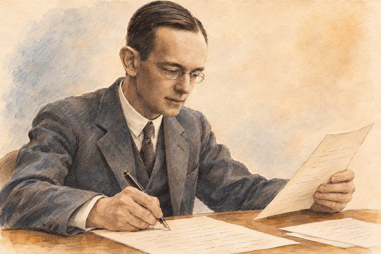
Fig. 15 — Illustrated evocation of Wilhelm Cauer writing his book on filter circuits around 1930–1931
His name remains associated with elliptic filters, but his contribution extends beyond that family: he helped turn filter design into a systematic calculation. This is precisely the path followed in this instalment: choose an overall response, then work out how to realise it.
Switched-capacitor filters: replacing a resistor with a clock
It is precisely as an integrated circuit that an elliptic filter is most often encountered—and this is down to a technique that has nothing to do with the mathematical approximations that precede. An integrated resistor is a poor component: it takes up a lot of silicon area, and its absolute value drifts by \pm 20\% from one batch to another. The technique that follows replaces it with a capacitor and two switches—that is, with less area and, as we shall see, with one more adjustment.
It is a technique that emulates a resistor by periodically transferring packets of charge with a capacitor and switches. Ideally, the capacitor does not dissipate energy as a resistor does, but the real switched circuit nevertheless consumes and dissipates energy.
The principle used is the one illustrated below. Switch S_1 is closed during time T_1 and open during time T_2. At the same time, S_2 is open during time T_1 and closed during time T_2. The period of one switching cycle, T, is equal to T_1 + T_2. The clock frequency, which is also the sampling frequency of the circuit, is F_s = 1/T—a single quantity, hence a single letter throughout this chapter, figures included. Voltages V_1 and V_2 are assumed to be ideal sources. Suppose V_1 > V_2. At the start of the cycle, S_1 is closed and S_2 open. Capacitor C therefore charges to voltage V_1. At instant T_1, S_1 opens and S_2 closes. The capacitor discharges down to voltage V_2. At instant T, the cycle repeats. During time T, charge has been transferred between input V_1 and output V_2. This charge—written \Delta q, so as not to confuse it with the quality factor Q—is equal to:
\Delta q = C\,(V_1 - V_2)
Since this transfer took place during time T, an equivalent current has therefore flowed between the two terminals:
I_{eq} = C\,(V_1 - V_2) / T = C\,(V_1 - V_2)\,F_s
Considering the equivalent resistive circuit:
I_{eq} = (V_1 - V_2) / R_{eq}
Over a duration T, this circuit is indeed equivalent to a resistor:
R_{eq} = \frac{1}{C\,F_s}
This formula holds only if the switching frequency F_s is large compared with the frequency of the signals V_1 and V_2 to be processed.
The illustration below is an example of application to an integrator. The integrator’s input resistor has been replaced by the equivalent switched-capacitor resistor. The same replacement can be applied to every resistor of an active filter.
Fig. 16 — Principle of switched-capacitor filters
The right-hand panel deserves a pause: the natural frequency of the integrator no longer depends on any absolute value. Its natural angular frequency is \omega_i = 1/(R_{eq}\,C_2) = F_s \cdot C_1/C_2, i.e. a natural frequency f_i = \dfrac{F_s}{2\pi} \cdot \dfrac{C_1}{C_2}: a clock frequency multiplied by a ratio of two capacitances. The factor 2\pi is not a presentational detail—it is what separates angular frequency from frequency, and confusing the two throws the tuning off by a factor of six. Now, two capacitors etched side by side on the same chip have an area ratio accurate to a few parts per thousand, whereas their absolute value drifts by \pm 20\%. It is this transfer of precision—from the value to the ratio—that makes integrated filters possible.
The switches are simply implemented with MOS transistors, and the control signals are derived from a non-overlapping two-phase clock, \Phi_1 and \Phi_2. This last adjective is not a specialist’s refinement: the whole operation of the circuit rests on it—and it incidentally forbids writing the second phase as \bar{\Phi_1}, because two signals that never overlap are precisely not complementary: there is an instant when both are at zero, and that is the whole point.
Fig. 17 — The non-overlapping two-phase clock and the two MOS switches it drives
If the two switches were closed together, even for an instant, V_1 and V_2 would be connected through two conducting MOS transistors: the charge would pass directly from input to output without going through C, and the equivalent resistance would no longer be 1/(C\,F_s). Hence the gap visible between the two pulses, during which both switches are open. It is paid for with a little extra logic—an inverter is not enough, two gates are needed to guarantee zero overlap—and it is the first of the hidden costs of this technique.
What is the point of such a system?
Replacing a resistor with a capacitor is, so far, still understandable. But adding two MOS transistors on top of that, which have to be driven by a two-phase clock, and so adding yet more logic to produce that clock—that is not exactly easy to understand!
And yet the benefit is considerable. Take as an example the order-5 low-pass filter from the chapter on Butterworth filters. Each of its sections has the same natural frequency, defined by f_0 = \frac{1}{2\pi\,RC} in this equal-component implementation. The Butterworth coefficients are obtained by adjusting the gain of each section. To move the cutoff frequency without changing the shape of the response, all the RC products involved must be varied simultaneously: the filter is therefore hard to tune with independent discrete components.
Now let us replace the resistors with switched-capacitor systems and put the whole thing in an integrated circuit. The space saving is already appreciable: the external circuitry can be limited to a few components and the clock generation.
The main benefit lies elsewhere, however. Let us go back to the definition of the equivalent resistance of the switched capacitor. This resistance depends first of all on the capacitor that has taken its place. So far, nothing unexpected: replacing a resistor with a capacitor leaves the value dependent on that capacitor. But above all—and this is the miracle of this type of filter—it depends on the switching frequency. From this observation, changing the clock frequency amounts to changing the cutoff frequency. And nothing prevents this from being done dynamically. Since the clock can be produced by a simple RC oscillator—that is the advantage of multivibrators—tuning can be achieved simply by replacing that resistor with a potentiometer.
Alas, every marvellous thing has its chink in the armour. This operating principle is based directly on sampling theory (the scent of analogue-to-digital and digital-to-analogue converters is not far off). And as such, a good number of problems are ready to arise. The first is linked to sampling itself. The signal is shaped into a staircase when it is stored in the capacitor, while the input signal continues to change (during phase T_2). To minimise this phenomenon, the sampling frequency must be as high as possible (the values commonly suggested are 50 and 100 times the cutoff frequency).
This hold is the first of the two defects inherent in sampling: the output is no longer a continuous curve but a series of steps, and these steps contain harmonics that the original signal did not have.
The second problem linked to this technique is called spectral folding (aliasing), and it is more serious, because it is irreversible.
After sampling, two frequencies separated by a multiple of F_s become indistinguishable. The observed frequency is |f_{in}-kF_s|, folded into the Nyquist interval [0,F_s/2]. Thus, with F_s=100\text{ kHz}, a component at 99\text{ kHz} folds back to 1\text{ kHz}. An anti-aliasing filter (an analogue filter placed before the sampler) must therefore sufficiently attenuate the components liable to fold back; no real filter removes them all at once beyond F_s/2.
The illustration below shows the same phenomenon with numbers that fit on a drawing—F_s = 10\ \text{kHz} and an input signal at 11\ \text{kHz}, which gives the same ghost at 1\ \text{kHz}. The input signal is drawn as a solid blue line, the ghost as a dotted red line.
Fig. 18 — Sampling, aliasing, and guard and smoothing filters
The fact to remember is one that the figure demonstrates rather than illustrates: the two sine waves pass through exactly the same sampling points. It is therefore not a measurement inaccuracy, nor a resolution defect that a better converter would correct: after sampling, the two signals are strictly the same set of numbers. No later processing can tell them apart—and that is why the anti-aliasing filter must be analogue, and placed before the sampler.
To guard against these two defects, two filters are needed: the first, placed at the input and usually called the guard filter, will attenuate sufficiently the frequencies above half the sampling frequency. The second, placed at the output and usually called the smoothing filter, will smooth out the staircases generated by the hold phase. The order required of these two filters is all the lower as the sampling frequency is far from the useful band: it is the width available between f_c and F_s/2 that gives the filter room to roll off. There is no simple proportion behind this rule—the number is read from the mask, as at the beginning of this part. This is what oversampling did, now standard in compact disc players: by sampling several times faster than the disc’s 44.1\ \text{kHz}, it moves half the sampling frequency away from the audio band, and replaces the very steep output filter that the gap between 20\ \text{kHz} and 22.05\ \text{kHz} would have required with a filter of much lower order.
But let us come back to our switched-capacitor filter: having to put another filter in front of it is something of a farce.
Another limiting criterion for this type of filter: to obtain a correct result, it is advisable to take the highest possible ratio between the clock frequency and the cutoff frequency—100, the higher of the two values quoted above. In the early 1990s, the clock of a common circuit such as the MF10 topped out at around 1\ \text{MHz}: with a ratio of 100, the passband of a low-pass filter therefore ended at about 10\ \text{kHz}. The rule itself has not changed: the useful band of a switched-capacitor filter is only a small fraction of its clock frequency.
Digital filters: once the signal is sampled, we might as well go all the way
The switched-capacitor filter has led us into an uncomfortable position: it samples the signal, suffers all the defects of sampling, requires one analogue filter upstream and another downstream—and in the end does nothing more than an analogue filter would have done. The next question follows naturally: since the signal is already cut into samples, why not convert it into numbers and let a computer do the filtering?
The missing word is out: in place of the switched capacitor, a computer. The signal enters through an analogue-to-digital converter, leaves through a digital-to-analogue converter, and in between there are no components left at all—only a sequence of numbers and a sequence of operations on them.
This shift changes the nature of the problem, which is why it closes this part rather than opening it: digital filtering is not limited to imitating an analogue filter. It can do so—and we shall see that it does so with the polynomials of this part—but it also performs processing that has no simple analogue equivalent, starting with a strictly linear phase, which not one of the four, Bessel, Butterworth, Chebyshev or Cauer, can produce. It is another discipline, that of signal processing, and what follows only shows its doorway.
The first obstacle was long the computation time: information was processed off-line, on recordings. Today it is processed on the fly, thanks to DSPs (Digital Signal Processors—computers whose instruction set is tailored to multiply-accumulate, the elementary operation of any digital filter) and the memories that accompany them.
The use of these filters has led to two new processing models:
Infinite impulse response (IIR) systems: because of their feedback loop, their response to an impulse theoretically goes on indefinitely, while decaying if the filter is stable.
Finite impulse response (FIR) systems: their response to an impulse contains only a finite number of samples, set by the number of filter coefficients.
High orders are possible, especially with FIR filters, but the useful order depends on the required performance, the sampling frequency, the latency and the available computing power.
These two terms describe a behaviour—what the filter does with an impulse. Three other terms describe the implementation, that is, the way the computation is wired, and the two sets are often confused:
Transversal, or non-recursive, implementation: the output signal depends only on the present value and the previous values of the input signal. This is the natural implementation of an FIR filter.
Recursive implementation: the output signal also depends on the previous values of the output. This is the natural implementation of an IIR filter.
Frequency-domain implementation by DFT (discrete Fourier transform): an FFT (fast Fourier transform) is an efficient algorithm for computing the DFT. Blocks of the signal are transformed, their spectrum is multiplied by the filter’s response, and an inverse DFT is then applied. In practice, block overlap must be managed to avoid discontinuities.
The two families, FIR and IIR, differ by a single line, literally: the presence or absence of a return path from the output to the input.
Fig. 19 — Structures of FIR and IIR digital filters, and all-pass phase-shift networks
In the transversal structure (top left), a sample enters, passes through a chain of shift registers—the z^{-1} blocks—each tap is multiplied by its coefficient, and the sum comes out. Nothing goes backwards: after N samples, the input has completely left the machine, and the impulse response stops. This is an FIR filter, always stable, because such a circuit has no way of sustaining itself.
Add the amber path—the output going back through a delay and returning to the adder—and everything changes. Today’s output depends on yesterday’s output, which depended on the day before’s: the impulse response never stops again; it merely decays if the coefficients allow it. This is an IIR filter, much more economical—it reaches a given order with far fewer coefficients—and whose stability has to be checked rather than assumed. It is exactly the same trade-off as between a passive filter and a feedback filter: feedback brings performance and takes away peace of mind.
The right-hand panel of the same illustration brings us to the last family of this study.
All-pass filters: selecting the phase, and the phase alone
Met in passing in Part One, all-pass filters are filters all the same: they select the phase rather than the magnitude.
A filter is described by two things: what it does to the magnitude of the signal and what it does to its phase. The four families in this part have all competed over the first; the last one gives up that contest entirely.
Its attenuation is indeed constant—and therefore, up to a scale factor, zero—whatever the frequency.
What it provides is a frequency-dependent phase shift—that is, a delay—hence their other, more telling name: phase-shift networks.
Their place in this part is no accident: they are the direct answer to the defect that Butterworth and Chebyshev confronted us with. A selective filter distorts the group delay (the delay undergone by the signal’s envelope); an all-pass, which touches no amplitude, can be placed after it to catch up on that delay where it is lacking. We do not correct the amplitude curve—it was the specification—we correct what the filter damaged while respecting it.
Fig. 20 — An all-pass after a Butterworth: the delay made up where it is missing
Just like the filters seen so far, these networks can be passive or active, first- or second-order.
1. First-order networks
First-order networks have a transfer function, a phase shift and a delay of the form:
F(p) = \frac{p - a}{p + a}
\phi(\omega) = \pi - 2\,\arctan(\omega/a)
\tau = \frac{2a}{a^2 + \omega^2}
Fig. 21 — First-order all-pass: a pole and its mirror-image zero, the phase and the delay
2. Second-order sections
Second-order sections have a transfer function of the form:
\text{with } u = \frac{\omega + b}{a} \quad\text{and}\quad v = \frac{\omega - b}{a}
Fig. 22 — Second-order all-pass: a delay hump you place and shape
These formulas say something remarkable, and it is worth naming it: the numerator and the denominator are conjugate. (p-a)^2 + b^2 and (p+a)^2 + b^2 have, for p = j\omega, exactly the same magnitude—hence a gain strictly equal to 1 at every frequency, not by approximation but by construction. Only the arguments differ, and it is this difference that becomes the phase shift. The circuit leaves the designer only the phase to adjust, because the amplitude is by nature beyond reach.
The operational-amplifier circuit in the previous illustration implements this first order: two equal resistors (R_1 = R_3) frame the amplifier, and it is the pair R_2\,C that sets a = 1/(R_2 C), hence the frequency at which the phase shift passes through 90° in absolute value. ⚠️ Up to the sign, precisely: this particular circuit gives F(p) = \dfrac{a - p}{a + p}, that is, the opposite of the canonical form written above. This can be checked at zero frequency, where the capacitor is an open circuit: the non-inverting input then sees the whole of V_{in}, the output is 2V_{in} - V_{in} = V_{in}, and the phase shift is therefore zero, not 180°. The phase starts at 0°, passes through -90° at \omega = a and tends towards -180°. The magnitude does not notice—it is 1 in both cases—but a phase-shift network is chosen for its phase, and a phase known only to within 180° is not a phase. Second-order passive networks, for their part, are built as lattices (two crossed branches, alternating L and C) or as bridged twin-T networks, and require no power supply—which remains an argument on a transmission line.
Conclusion
We set out from a very concrete annoyance: two correct sections, placed end to end, gave a filter whose passband had shrunk without warning. The answer fits in one sentence, and it has taken up this whole part—a filter of order n is not made by copying a section n/2 times; we start from the polynomial of the desired response and factor it. Each section then receives its own natural frequency and Q, none of which is that of the complete filter, and some of which are even frankly bad taken in isolation.
What remains is the question this part has asked four times under four names: what shape should the knee have? None of the four families wins, and that is the most useful result to take away.
Butterworth never moves its -3\text{ dB} point as the order goes up, and its passband is the flattest. It is the default choice, the one we make when the specification says nothing more.
Bessel makes the group delay as flat as possible, and a signal with edges comes out of it with its shape intact. The price is paid in rejection: 16\ \text{dB} less than Butterworth one octave up.
Chebyshev spends the ripple allowed in the passband to sharpen the knee. Its downside is not the overshoot—almost the same as Butterworth’s—but the duration of the resonance, twice as long.
Cauer also spends the ripple allowed in the stopband, and digs transmission zeros into it. It meets a mask at order 5 where Butterworth requires order 24; in exchange, it demands tight-tolerance components and a phase that one gives up defending.
Two ancillary techniques have been grafted on. Switched capacitors make the cutoff tunable by a simple clock frequency, in exchange for all the defects of sampling—including an analogue filter to be placed in front, which is not without irony. And digital filtering, which takes the same logic all the way.
On this last point, in the early 1990s these techniques were beyond the reach of the amateur, and their cost made them unsuitable for most needs. That is no longer the case: a microcontroller costing a few euros now runs, in real time and on several channels, filters of orders that would then have been considered spectacular. What has not changed, on the other hand, is all the rest of this part: the Butterworth, Bessel and Chebyshev polynomials are used in exactly the same way to design a digital filter—the analogue prototype is calculated, then transposed. The choice of family, for its part, still has to be made in full, and it is made with the same arguments.
Analogue filtering has not disappeared either, for a reason that has nothing to do with nostalgia: the anti-aliasing filter of any sampled system is, and will remain, analogue. There is no digital without an analogue filter in front.
We now know how to give a filter the shape we want. In the next article, we will explore audio applications: RIAA equalisation for vinyl records, loudness compensation and the Baxandall tone control. We will then change the question: instead of seeking the response closest to an ideal, we will start from deliberately shaped curves, where that shaping is precisely what we want to achieve.
Sources and background
Main inspiration. “Les filtres passifs et actifs”, Part Three, by Emmanuel Deret, Hobbytronic No. 13, pp. 2–9. Emmanuel Deret was editor-in-chief and one of the principal contributors to this French electronics magazine of the early 1990s. The original issues can be consulted at abandonware-magazines.org.
Primary sources.
Stephen Butterworth, “On the Theory of Filter Amplifiers”, Experimental Wireless and the Wireless Engineer, vol. 7, October 1930, pp. 536–541.
Friedrich Wilhelm Bessel, “Untersuchung des Theils der planetarischen Störungen, welcher aus der Bewegung der Sonne entsteht”, Abhandlungen der Königlichen Akademie der Wissenschaften zu Berlin, 1824, pp. 1–52—the systematic study of the functions that bear his name.
Pafnuty Chebyshev, “Théorie des mécanismes connus sous le nom de parallélogrammes”, Mémoires des savants étrangers présentés à l’Académie impériale des sciences de Saint-Pétersbourg, vol. VII, 1854, pp. 539–568.
W. E. Thomson, “Delay Networks Having Maximally Flat Frequency Characteristics”, Proceedings of the IEE, part III, vol. 96, no. 44, November 1949, pp. 487–490.
Anatol I. Zverev, Handbook of Filter Synthesis, Wiley, 1967—for the polynomial tables and the f_{-3\text{dB}}/f_0 correspondences of Bessel filters.
Analog Devices, Basic Linear Design (ed. Hank Zumbahlen), chapter 8, “Analog Filters”—Butterworth, Bessel and Chebyshev poles, and construction of the ellipse.
Alan V. Oppenheim and Ronald W. Schafer, Discrete-Time Signal Processing, 3rd edition, Pearson, 2010, for sampling, FIR/IIR filters and the DFT.
Numbered references for the historical notes and portraits
This list brings together the identified sources for the four historical notes, along with those used to check the captions and illustrations. Each number points to the document or its catalogue entry and explains what it establishes. The image descriptions were checked on 4 November 2026; information missing from a source is not reconstructed as fact.
<a id=”source-historique-1″></a> Sescosem — industrial context in 1972. Larousse, Journal de l’année 1972, “Productions — La crise des composants”. Contemporary source on the component market and discussions of a merger with Telefunken and Plessey.
<a id=”source-historique-2″></a> Sescosem — brands, factories and components. The CPU Shack Museum, “SESCOSEM and the French 6800”, 14 May 2017. History of SESCO and COSEM, manufacturing sites and changes in markings. The museum’s SESCOSEM topic index provides another route to the article.
<a id=”source-historique-3″></a> From SGS-Thomson to STMicroelectronics. STMicroelectronics, corporate FAQ, section on the company’s origins. The company’s own source for the 1987 merger and the name change in May 1998.
<a id=”source-historique-4″></a> Bessel — career and astronomical work. J. J. O’Connor and E. F. Robertson, “Friedrich Wilhelm Bessel”, MacTutor, University of St Andrews. Biographical account of Königsberg and Bessel’s mathematical and astronomical work.
<a id=”source-historique-5″></a> Bessel — original portrait. Wikimedia Commons, catalogue entry for “Friedrich Wilhelm Bessel (1839 painting)”. Christian Albrecht Jensen, 1839, oil on canvas, 25 × 21 cm; Ny Carlsberg Glyptotek, Copenhagen. Provenance and public-domain status of the reproduction.
<a id=”source-historique-6″></a> Bessel — origin of the polynomials’ name. H. L. Krall and Orrin Frink, “A New Class of Orthogonal Polynomials: The Bessel Polynomials”, Transactions of the American Mathematical Society, vol. 65, no. 1, 1949, pp. 100–115. Original publication distinguishing the polynomials from the functions studied by Bessel.
<a id=”source-historique-7″></a> Bessel–Thomson — application to delay networks. W. E. Thomson, “Delay Networks Having Maximally Flat Frequency Characteristics”, Proceedings of the IEE — Part III: Radio and Communication Engineering, vol. 96, no. 44, November 1949, pp. 487–490. Original publication on maximally flat delay networks; the DOI points to the publisher’s entry and does not guarantee free access to the full text.
<a id=”source-historique-8″></a> Chebyshev — mechanisms and approximation. P. Tchébychef, “Théorie des mécanismes connus sous le nom de parallélogrammes”. Copy digitised by ETH-Bibliothek Zürich, shelfmark Rar 23506, dated 1853 in the catalogue; persistent identifier. This is distinct from the reference to volume VII of the Mémoires, published in 1854, pp. 539–568, cited above. Primary source on the mechanical problem leading to approximation.
<a id=”source-historique-9″></a> Chebyshev — biographical context. J. J. O’Connor and E. F. Robertson, “Pafnuty Lvovich Chebyshev”, MacTutor, University of St Andrews. Career in Saint Petersburg, interest in mechanisms and work on approximation.
<a id=”source-historique-10″></a> Chebyshev — original portrait. Wikimedia Commons, description of “Chebyshev.jpg”. The description dates the portrait to the 1890s and classifies it as public domain. It identifies neither the photographer nor the original collection: attribution to the Russian Academy of Sciences cannot therefore be inferred from this entry.
<a id=”source-historique-11″></a> Cauer — research and context of the illustrated scene. Emil Cauer, Wolfgang Mathis and Rainer Pauli, “Life and Work of Wilhelm Cauer (1900–1945)”, MTNS 2000, Perpignan, pp. 1–2 and 5. Study including his son’s testimony; source for the 1926 thesis, the network synthesis programme and the completion of Siebschaltungen during the American stay in 1930–1931. The book was published by VDI-Verlag, Berlin, in 1931. This source documents the activity depicted, not the desk’s appearance or Cauer’s pose.
<a id=”source-historique-12″></a> Cauer — family portrait of 4 September 1930. Wikimedia Commons, description of “Wilhelm Cauer 1930-09-04.jpg”. The uploader states that their grandfather was photographed by his own father, Wilhelm Cauer, and that the picture was subsequently scanned and cropped. Uploaded on 6 March 2019; public domain according to the description. The 2019 date concerns the digital file, not the photograph taken in 1930. Location and occasion unspecified.
Picture credits
The three portraits reproduce historical documents: their attributions and status are given in references 5, 10 and 12. The copyright on this article’s original creations does not apply to these archive documents.
This site uses Google services that set cookies: you can accept or decline them. Our own visit counter only sets a cookie if you accept. It records your IP address in every case.