




Filters with unfamiliar names
Pre-emphasis, de-emphasis, weighting, equalisation: audio filters have rather forbidding names, yet we have all used them without knowing it. They are what makes the difference between an ordinary device and one described as “high fidelity”.
They exist because nothing is perfect. Neither sensors, such as microphones and playback heads, nor reproduction devices, such as loudspeakers and screens. Nor human beings themselves, with their ears and eyes. Each has a limited operating range, and imperfections within that range. Audio filters aim to obtain a consistent result from one end to the other.
In audio, the limits are those of human hearing: roughly 16\text{ Hz} to 20\text{ kHz}. But the ear is not an impartial judge within those limits. At moderate levels, it is most sensitive between approximately 2 and 5\text{ kHz}, and its sensitivity falls at low and very high frequencies, increasingly so at low sound levels. The 1\text{ kHz} signal used to characterise amplifiers is a convenient measurement convention; it does not mark the ear’s peak sensitivity. We can regard the ear as a rather poor band-pass filter (a filter that passes only a range of frequencies), provided we do not take the analogy too far.
Weighting: a filter that imitates the ear
Weighting filters arose from this observation. A sound level meter displaying the raw sound pressure of a noise would not accurately convey how the ear perceives it: a 50\text{ Hz} hum and a 3\text{ kHz} whistle at the same sound pressure are not equally disturbing. The meter therefore places a standardised filter ahead of its detector to imitate the ear, and displays dB(A) or dB(C), depending on the selected filter.

A weighting was originally modelled on the ear’s sensitivity to quiet sounds. It attenuates by 30.3\text{ dB} at 50\text{ Hz} and 19.1\text{ dB} at 100\text{ Hz}. C weighting, modelled on loud sounds, is nearly flat between 31.5\text{ Hz} and 8\text{ kHz}. Both are ordinary filters defined by IEC 61672-1: six poles (factors in the denominator of the transfer function) and four zeros at the origin for A weighting, four poles and two zeros for C weighting. The difference between the two readings of the same noise indicates its low-frequency content: 29\text{ dB} for a pure 50\text{ Hz} hum. We will encounter this level-dependent sensitivity again with loudness compensation.
The other three families
The second observation can be made with an oscilloscope. Connected to an amplifier playing music, it shows a waveform dominated by bass. Its amplitude is substantial, whereas the midrange and, even more so, the treble have much smaller amplitudes. These differences become a problem when recording sound on a medium (disc, magnetic tape or radio waves) and then recovering it. Hence the second family: pre-emphasis and de-emphasis filters. They work in pairs: the first adjusts the relative amplitudes before the medium, and the second restores the original amplitudes during playback.
The third family, equalisation filters, deals with what remains. The frequency responses of sensors and loudspeakers are far from flat, and the listening room’s response is no flatter. A room lined with curtains does not damp sound like one with bare walls: different corrections are needed to hear the same result.
Finally, there is the family studied in the first three parts: filters whose purpose is simply to filter. Two-way and three-way loudspeakers are typical examples, with crossover filters dividing the spectrum between the drivers.
Building a response to order
In Part Three, a high-order filter was obtained by cascading sections of the same type, such as low-pass sections, until the desired order was reached. Equalisation networks follow the same principle, with one difference: their sections are of different types and have different corner frequencies.
We start with the response specification, meaning its characteristic points: the frequencies at which the slope changes, and the value of each slope. We then work backward from the desired response. Each frequency at which the slope turns downward becomes a pole (a factor in the denominator of the transfer function). Each frequency at which it turns upward becomes a zero (a factor in the numerator). The gains of these factors add in decibels, as do their slopes: a slope of -20\text{ dB} per decade followed by an upward change of +20\text{ dB} per decade leaves a zero slope, or a plateau.
Take the simplest equalisation: more gain in the bass, less in the treble, without eliminating either region. This is a shelving response. A low-pass followed by a high-pass would not produce it: the first attenuates the highest frequencies, the second the lowest, and their cascade produces a band-pass. We need a pole followed by a zero, hence a network whose gain remains nonzero at both ends.

In the circuit shown, R_1 is in series with the input; the R_2–C branch runs to ground. The ideal operational amplifier draws no input current. At low frequencies, the capacitor almost blocks the current: the voltage drop across R_1 is small, and the non-inverting input receives almost V_e. At high frequencies, the capacitor behaves almost like a wire: R_1 and R_2 form a voltage divider.
The amplifier multiplies this voltage by K=1+R_f/R_g=31. The overall gain is:
The denominator factor introduces the pole, which bends the slope downward here, associated with f_1=1/[2\pi(R_1+R_2)C]\approx49.74\text{ Hz}. The numerator factor introduces the zero, which bends it upward, associated with f_2=1/(2\pi R_2C)\approx159.15\text{ Hz}. Such a zero must not be confused with a complete high-pass filter, which also has a denominator.
With R_1=22\text{ k}\Omega, R_2=10\text{ k}\Omega and C=100\text{ nF}, the gain tends towards 31, or 29.83\text{ dB}, at low frequencies; at high frequencies, it tends towards 31\times10/32=9.6875, or 19.72\text{ dB}. The standard component values therefore give a difference of 10.10\text{ dB} between the plateaus, close to the intended 10\text{ dB}.
The contributions of the factors multiply; their gains in decibels and their phases add. Straight lines with slopes of -20 and then +20\text{ dB} per decade serve as approximations far from the transitions. Here, f_1 and f_2 are close together: the actual curve has no long segment at -20\text{ dB} per decade, and approaches its plateaus gradually.
This multiplication cannot be applied blindly to interconnected passive circuits: loading by the following circuit can change the response of the preceding one, as shown in Analog Devices’ study of cascaded RC sections. In our example, the amplifier’s ideal input avoids this loading.
All the responses in this part are built this way. The most famous of them is cut into every vinyl record.
Vinyl records and the RIAA curve
A cartridge that measures velocity
Of all equalisers, the RIAA preamplifier is probably the best known and most widely used. It amplifies and equalises the signal from magnetic turntable cartridges.
Not all cartridges require the same preamplifier. Ceramic or piezoelectric cartridges can deliver hundreds of millivolts, but they require a high-impedance input (one that draws little current) and a load suited to their response: an arbitrary auxiliary input will not necessarily do. An MM, or moving-magnet, cartridge might deliver 5\text{ mV} at a modulation velocity of 5\text{ cm/s}; MC, or moving-coil, models may deliver much less and require more gain. Both are velocity sensors: their voltage depends on how quickly the stylus moves in the groove, rather than on the amplitude of that movement. Their sensitivity is therefore expressed in millivolts per centimeter per second; our MM example has a sensitivity of 1\text{ mV} per \text{cm/s}.
Designing a magnetic-cartridge preamplifier requires knowing the maximum modulation velocity. This is the velocity of the stylus oscillating across the groove (the modulation velocity), not the speed at which the groove travels beneath it. Application handbooks of the period give design maxima: 21\text{ cm/s} for a stereo record in Signetics’ Analog Applications (1979, page 209), and 25\text{ cm/s} between 800 and 2500\text{ Hz} in National Semiconductor’s Audio/Radio Handbook (1980). In practice, good-quality recordings use velocities of 3 to 5\text{ cm/s}, but measurements of commercial records have revealed much higher peaks (Tomlinson Holman, 1977).
Why cut a deliberately altered response?
This velocity-sensitive pickup has an immediate consequence for disc cutting. At a given modulation velocity, the amplitude of the stylus displacement is inversely proportional to frequency: at 20\text{ Hz}, it is fifty times greater than at 1\text{ kHz}. Bass cut at full velocity would require grooves so wide that they overlapped, and a record side would hold only a few minutes of music. Bass is therefore deliberately attenuated during cutting to save space and extend playing time.
Treble presents the opposite problem. Every analogue device generates background noise, and high-frequency signals have very small amplitudes: they are often harmonics of lower-frequency sounds. During playback, they could be buried in groove noise. They are therefore boosted during cutting to keep them above that noise.
The signal written into the groove is thus altered in two ways, and playback must apply the inverse corrections. To allow any record to be played on any turntable, these changes were standardised: this is the RIAA response, named after the Recording Industry Association of America.

The RIAA playback response boosts bass and attenuates treble relative to the 1\text{ kHz} reference: it reverses the cutting process. The slope changes are gradual: there is no plateau at exactly 0\text{ dB} between 500 and 2122\text{ Hz}. The ideal response is approximately +19.27\text{ dB} at 20\text{ Hz}, +2.65\text{ dB} at 500\text{ Hz}, and -19.62\text{ dB} at 20\text{ kHz}: these account for the 39\text{ dB} in the introduction.
To calculate the curve and its phase shift, we use:
Here, s=j2\pi f, where f is frequency in hertz. Dividing by the magnitude at 1\text{ kHz} sets the gain to 0\text{ dB} at that frequency without changing the phase. The frequencies f_i=1/(2\pi\tau_i) mark the transitions of the individual factors in the formula; they do not represent three overall gain cutoffs at the −3 dB point.
The three standardised RIAA time constants are:
- \tau_1 = 3180\ \mu\text{s} \implies f_1 = \frac{1}{2 \pi \times 3180 \times 10^{-6}} \approx 50.05\text{ Hz}
- \tau_2 = 318\ \mu\text{s} \implies f_2 = \frac{1}{2 \pi \times 318 \times 10^{-6}} \approx 500.5\text{ Hz}
- \tau_3 = 75\ \mu\text{s} \implies f_3 = \frac{1}{2 \pi \times 75 \times 10^{-6}} \approx 2122\text{ Hz}
The response specification can therefore be read just as in the previous section: a pole at 50\text{ Hz}, a zero at 500\text{ Hz}, and a pole at 2122\text{ Hz}. The slopes of 20\text{ dB} per decade tell us that first-order sections suffice, each built from a resistor–capacitor pair whose product equals the time constant: \tau = RC = 1/(2\pi f).
The preamplifier
Besides equalisation, RIAA preamplifiers must provide enough signal gain to reach a level compatible with the amplifier’s input sensitivity.

The circuit is non-inverting: the signal reaches the + input and the feedback network returns to the - input. Its topology is described in Analog Devices, Op Amp Applications, Chapter 6, Figures 6-9 and 6-10. The values shown here belong to our example; they are not copied from the handbook.
The two networks R_1\parallel C_1 and R_2\parallel C_2 are connected in series between the output and the inverting input. Using their impedances (frequency-dependent opposition to current), we obtain:
The angular frequency \omega equals 2\pi f. The calculation therefore includes the shunt-leg capacitor C_g=220\ \mu\text{F}, resistor R_g=150\ \Omega, and the +1 term of the non-inverting circuit.
The network products are R_1C_1=3196\ \mu\text{s} and R_2C_2=72.8\ \mu\text{s}. Its intermediate time constant is (R_1\parallel R_2)(C_1+C_2)=310.43\ \mu\text{s}: these values approximate the RIAA constants without matching them exactly. The full gain also depends on the shunt leg.
With an ideal operational amplifier and the nominal values shown, the gain at 1\text{ kHz} is 33.86\text{ dB}, or approximately 49.31 in voltage: an input of 3\text{ mV} produces about 148\text{ mV}. After normalising both curves to 0\text{ dB} at 1\text{ kHz}, the difference between the circuit and the reference ranges from -0.19 to +0.34\text{ dB} over 20\text{ Hz} to 20\text{ kHz}. This is a nominal calculation, not a guarantee that includes tolerances.
The shunt-leg capacitor C_g sets none of the three RIAA time constants, but adds a transition at very low frequencies. At DC it opens the shunt leg: the gain applied to the offset voltage (the op amp’s small internal DC error) falls to 1, instead of approximately 492 if R_g were connected directly to ground. Input bias currents can nevertheless produce additional DC offsets. The frequency 1/(2\pi R_gC_g)\approx4.8\text{ Hz} identifies this shunt-leg transition. Its effect is not entirely negligible at 20\text{ Hz}: the calculation gives about 0.24\text{ dB} of additional attenuation compared with the same circuit with C_g shorted. This effect is included in the curves and in the deviation quoted above.
The MM (moving-magnet) cartridge sees a resistance of 47\text{ k}\Omega here. The total capacitance C_{\mathrm{tot}} includes the cable, the amplifier input, and any added capacitor: its value must be chosen from the cartridge’s specifications, and is not universally 100 to 200\text{ pF}. The curves start from the voltage V_e already present at the input; they do not include the cartridge’s own response. The drawing shows the equalisation stage, with power supplies and decoupling omitted.
Gain is chosen to match two sensitivities: that of the cartridge to be amplified, and that of the amplifier input to be driven. A cartridge rated at 1\text{ mV} per \text{cm/s}, played at 5\text{ cm/s}, produces 5\text{ mV}; multiplied by 49.31, this becomes approximately 247\text{ mV}, enough to drive an amplifier’s auxiliary input, whose sensitivity is typically in the hundreds of millivolts.
Three ways to distribute the time constants
There are many RIAA preamplifier circuits, distinguished mainly by how they distribute the three time constants.
The inverting arrangement places the two sections in the feedback path of an amplifier whose + input is grounded. Its input resistor then sets the load seen by the cartridge, and adds its own noise to the weakest signal in the entire chain. The non-inverting circuit in our example avoids this drawback.
The four components in the two RC networks allow all three feedback-network time constants to be chosen. If \tau_1=R_1C_1 and \tau_3=R_2C_2, the zero’s time constant is \tau_2=(R_2\tau_1+R_1\tau_3)/(R_1+R_2). We can therefore target 3180, 318 and 75\ \mu\text{s} by choosing, in particular, R_1/R_2=(3180-318)/(318-75)\approx11.78. The deviations in our example arise from the selected standard values and the full function 1+Z_f/Z_g, not from an inability to obtain three time constants with two networks. Another solution distributes the equalisation: a first active stage implements 3180 and 318\ \mu\text{s}, then a passive RC network between two stages implements 75\ \mu\text{s}. This separates adjustment of the treble transition from the other two, provided the next stage does not load the network. Gain must then be distributed with noise and overload margin in mind: adding stages or reducing the gain of each does not automatically reduce noise or distortion.
Magnetic tape and the NAB curves
If RIAA stood for the turntable, NAB (National Association of Broadcasters) stands for the tape recorder. And with it, the difficulties begin.
Tape hisses and saturates
The problem is different from that of the disc. Magnetic tape is an excellent noise generator. The head’s own noise is joined by noise associated with erasure and bias (a high-frequency signal added during recording to improve linearity). As an indication of scale, Revox currently specifies noise below -70\text{ dB} for its B77 MK III tape recorder, at both 19 and 38\text{ cm/s}, relative to the recording level that produces 2.5\ \% distortion. This is the performance of one model under its stated measurement conditions, not a limit applicable to all machines. Hiss is most troublesome at high frequencies, where Dolby noise-reduction systems concentrate their action. Studio Dolby A divides the spectrum into four bands: a low-pass at 80\text{ Hz}, a band-pass from 80\text{ Hz} to 3\text{ kHz}, and two overlapping high-pass bands, one above 3\text{ kHz} and the other above 9\text{ kHz}. Cassette Dolby B acts only at high frequencies, using a single band whose cutoff frequency shifts with the signal, for an effect of up to approximately 10\text{ dB} (Ray M. Dolby and Stanley G. Cossette, US Patent 5,185,806). To keep the treble from being lost, it is boosted during recording and reduced during playback. Tape noise, which was not boosted, is reduced along with it.
Pre-emphasis nevertheless has a limit. Beyond a certain amplitude, the tape saturates: it can no longer reproduce an increase in signal proportionally. The pre-emphasis region therefore cannot cover the entire frequency range. And unlike disc recording, bass is not attenuated during recording: it would have to be boosted during playback, bringing low-frequency noise up with it. Since a tape recorder both records and plays back, it contains both filters of the pair: a pre-emphasis filter for recording and a de-emphasis filter for playback.
Playback
The playback head’s output voltage varies with frequency even at constant magnetic flux on the tape, so the preamplifier must also correct this response. The electrical playback-gain curve must not be confused with the recorded-flux curve.
The NAB curves were established for open-reel tape recorders. The cassette complicated matters somewhat, and the video recorder complicated them further. An equalisation curve depends on two criteria: tape speed (38.1, 19.05, 9.53, 4.76 or 2.38\text{ cm/s}) and tape formulation (ferric oxide, chromium dioxide, ferrichrome or metal). Each combination has its own curve. The cassette provides a good example. The 1968 Philips standard specified two playback time constants, 1590 and 120\ \mu\text{s}, for ordinary ferric-oxide tape. In July 1972, “high-resolution” chromium-dioxide tapes received their own constants, 3180 and 70\ \mu\text{s}, in an addendum to IEC Publication 94A. The DIN standard subsequently set the bass time constant to 3180\ \mu\text{s} for both types (Nakamichi, Technical Bulletin 2: Playback Equalization). Playing chrome tape with the ferric setting therefore raises the treble by a few decibels.
The figure compares two references from Signetics’ Analog Applications handbook, 1979, page 218: 3180/50\ \mu\text{s} at 19.05 and 38.1\text{ cm/s}, and 3180/90\ \mu\text{s} at 9.525\text{ cm/s}. Europe uses the CCIR convention, subsequently adopted by the IEC, at the same speeds: 70\ \mu\text{s} at 19\text{ cm/s} and 35\ \mu\text{s} at 38\text{ cm/s}. A recorder intended for use on both sides of the Atlantic therefore offers both, as does today’s Revox B77 MK III.
To make the curves easier to compare, their high-frequency plateau has been set to 0\text{ dB}: this normalisation removes a constant gain so that their shapes can be compared. The ideal responses approach a plateau at low frequencies, fall at approximately 20\text{ dB} per decade in the intermediate region, then approach the high-frequency plateau. The transitions are gradual, around 50\text{ Hz} and then 3183\text{ Hz} for 50\ \mu\text{s}, or 1768\text{ Hz} for 90\ \mu\text{s}. With a slope of 20\text{ dB} per decade, simple RC sections suffice, one in series and one in parallel.

The playback circuit follows the NAB branch in Philips application note AN142, Figure 14. Between the output and the inverting input, 1.1\text{ M}\Omega is in parallel with a branch consisting of 16\text{ k}\Omega in series with 3\text{ nF}. Towards ground, 1.1\text{ k}\Omega is in series with 20\ \mu\text{F}. This last capacitor reduces the gain at very low frequencies.
The red curve is calculated using these values and an ideal operational amplifier. It approaches the 3180/50\ \mu\text{s} reference without reproducing it exactly. Its high-frequency voltage gain, approximately 15.34, has been removed for comparison. The input voltage V_e is taken after the coupling capacitor, at the non-inverting input: the head’s own response and its load are therefore not included.
One practical detail distinguishes playback circuits: their turn-on time. In a single-supply amplifier, DC bias often passes through a large resistor and a large capacitor, and the preamplifier operates normally only once that capacitor has charged. National Semiconductor’s 1976 audio handbook gives the formula:
The capacitor need not charge fully: it only has to reach 2.4\text{ V}, one tenth of a 24\text{ V} supply, which takes about one tenth of the R_4C_2 time constant. With 2.2\text{ M}\Omega and roughly twenty microfarads, this constant exceeds 40\text{ s}, so the handbook’s typical playback preamplifier takes approximately 5\text{ s} to become operational. Increasing the supply voltage or reducing the gain shortens this delay; a “fast turn-on” version, adding a second pole to the bias network, reduces it to 0.1\text{ s}.
Recording
Recording adjustments must account for the head, the tape, its losses and its saturation. They cannot be reduced to simply inverting the electrical playback gain.
The lower detail comes from Signetics 1979, Figure 8-52, page 214. Bias is a high-frequency signal added to improve recording. The bias trap consists of an inductor and capacitor in parallel; this combination is inserted in series in the audio path. At its tuned frequency, it strongly opposes the return of the bias signal to the amplifier. The recording head is current-driven, and the 200\text{ k}\Omega resistor sets this current: in the worked example in National Semiconductor’s audio handbook (1976), 6\text{ V} RMS for a head requiring 30\ \mu\text{A} gives precisely 200\text{ k}\Omega. Since the trap’s inductor and capacitor values are unspecified, this drawing does not guarantee tuning to the bias frequency, which the same handbook places typically around 70\text{ kHz}. The head, its return path and the bias injection are outside this detail.
These simple filters are found in all conventional tape recorders. The desire to improve the signal-to-noise ratio further then led to noise-reduction systems: Dolby, dbx and High Com. The first Dolby system, intended for studios, reduced hiss by 10 to 15\text{ dB} (Walter G. Salm, Radio-Electronics, October 1969). These are no longer simple filters. Their processing depends on the signal’s amplitude as well as its frequency, during both recording and playback. They therefore cannot be described by a single amplitude-independent linear-filter response.
FM radio: the same pair, over the air
Frequency-modulated transmission applies the same principle, again to improve the signal-to-noise ratio. After demodulation, an FM receiver’s noise increases with frequency: extra margin is needed precisely in the treble.
Treble pre-emphasis is therefore applied at the transmitter, before the modulation stage. Its standardised time constant is 50\ \mu\text{s} in Europe, Japan and most countries, corresponding to f_c \approx 3183\text{ Hz}, and 75\ \mu\text{s} in the Americas and South Korea, corresponding to f_c \approx 2122\text{ Hz}. The inverse correction is applied at the receiver.

The de-emphasis circuit is simply a first-order low-pass filter: a series resistor and a capacitor to ground, whose product RC equals the standardised time constant. The figure shows what makes a pair: pre-emphasis 1+j\tau\omega and de-emphasis 1/(1+j\tau\omega) have opposite gains in decibels and opposite phases, and their product is exactly 1. The music therefore emerges intact; noise added during the radio transmission passes only through the second half and emerges attenuated. The two halves must, however, follow the same standard: a 50\ \mu\text{s} receiver receiving a 75\ \mu\text{s} transmission leaves 2.8\text{ dB} of excess treble at 5\text{ kHz}.
Equalisation filters
The filters considered so far work in complementary pairs: what one changes, the other restores. No significant difference remains between the source signal and the reproduced signal, and the size of any residual difference measures the device’s fidelity.
With equalisation filters, the change to the signal is permanent: no later filter will undo it. They serve two purposes:
- The first is to compensate for a sensor or reproduction device’s shortcomings. In this case, they flatten the frequency response of the complete system.
- The second is more subjective: making a signal more pleasant to listen to or view. Here, no rule determines which setting is best.
This category includes many devices. The most widespread sits on the front panel of almost every amplifier.
Tone controls
Of all these devices, the tone control is the most commonly encountered. It changes the response to increase or decrease the signal amplitude in the bass or treble, according to the listener’s taste. Its response looks somewhat like that of the RIAA preamplifier, with a plateau, a slope and another plateau, but here the listener moves the plateaus.
Passive sections and their cost
The most traditional basic sections are entirely passive: each uses a potentiometer, two capacitors and two resistors. The principle still relies on RC sections whose corner frequencies move with the wiper position. The figure uses the worked example from National Semiconductor’s 1976 audio handbook: \pm20\text{ dB} of adjustment at 50\text{ Hz} and 10\text{ kHz}, with a 100\text{ k}\Omega logarithmic potentiometer.

In the bass section, each half of the track is bypassed by its capacitor as frequency rises. At high frequencies, only the divider formed by R_{12} and R_{11} remains, unaffected by the wiper position. At low frequencies, the capacitors cease to act, and the wiper selects the transmitted fraction: almost the entire signal at the top, almost nothing at the bottom.
The treble section is the same arrangement with resistors and capacitors interchanged. C_{12} and C_{11} flank the track; R_{14} and R_{15} connect its two ends to the wiper. At low frequencies, the two capacitors alone form a divider, unaffected by the wiper. At high frequencies they behave like wires, and the divider consists of R_{14}, R_{15} and the two portions of the track. The values follow a rule: the track resistance must be much greater than R_{14}, which must itself be much greater than R_{15} (100, 10 and 1\text{ k}\Omega). The fixed resistors, rather than the track, then set the corner frequencies and the amount of adjustment: the ratio R_{15}/R_{14}, equal to C_{12}/C_{11}, is 1/10, or 20\text{ dB}. This can be seen in the mid-track curve, which deviates from flat by only 1.3\text{ dB}. A cheaper version omits R_{14} and R_{15}, but the cut corner then shifts upward by a decade. An asymmetry remains in either case: at full cut, the treble continues to fall, without the plateau that limits the boost.
The figure also shows the price of this simplicity. At the flat setting, each section divides the signal by 11, or -20.8\text{ dB} at all frequencies: it is a permanent voltage divider, and the signal must subsequently be amplified again. This flat setting is not halfway along the track, but at 9.1\ \% of its length from the grounded end. This is why these sections use logarithmic potentiometers: halfway through their travel, the wiper divides the track into 90\ \% and 10\ \%, hence the labels 0.9 and 0.1 beside the wiper in the schematics. On either side, the adjustment reaches approximately \pm20\text{ dB}. In the bass section, the corners move with the wiper; in the treble section, R_{14} and R_{15} hold them in place.
All these curves also assume an unloaded output. According to the same handbook, a load equal to one tenth of the track resistance is enough to shift the treble section’s corners by a decade. The section must therefore drive a high-impedance input stage, which also restores the lost 20.8\text{ dB}.
Active tone controls address both drawbacks at once.
The active Baxandall tone control
Peter Baxandall published his famous feedback tone control in 1952. The original circuit used a valve amplifier; the circuit shown here is a later op-amp adaptation, with a symmetrical network in the feedback loop. The network no longer acts as a divider in the signal path: it sets the amplifier gain, which is -1 with both controls centred. There is no loss to recover.

The network shown follows one channel of Texas Instruments application note SLOA042, Figure 3, adapted to a 0\text{ V} reference with dual supplies. The application’s input buffer is omitted. Both potentiometers are 100\text{ k}\Omega. The 3.3\text{ k}\Omega resistor connects the treble wiper to the inverting input; the two 3.3\text{ nF} capacitors connect to the ends of its track.
With both tracks centred, the ideal model gives exactly V_s/V_e=-1: the magnitude is unchanged, or 0\text{ dB}, but the signal is inverted. The phase graph shows the additional variation relative to this 180^\circ inversion. Component tolerances, source resistance and amplifier limitations can alter the actual response.
The curves are calculated from the components shown, with one potentiometer moved to an end stop and the other held at the centre:
- The bass potentiometer P_1 gives approximately \pm16.73\text{ dB} at 50\text{ Hz}.
- The treble potentiometer P_2 gives approximately \pm15.82\text{ dB} at 15\text{ kHz}.
- There is no shared pivot frequency fixed at exactly 1\text{ kHz}: the corrections are small there, but not all zero.
The two controls share the inverting input and interact. Their effects therefore do not combine like those of two fully independent equalisers.
Three bands: the midrange joins in
Combining these sections with a third, centred in the middle of the spectrum, produces a three-band tone control: bass, midrange and treble. Bass and treble retain their shelves; the midrange has a bell-shaped response. With all potentiometers centred, the response is flat. With bass and treble at maximum and the midrange centred, it becomes a valley; with bass and treble at minimum, it becomes a hill. Turning up the midrange alone raises a hill in the centre; turning it down creates a dip.
The presence filter
Although a two-band tone control adjusts bass and treble, both important components of music, it does not act directly on the midrange.
This range contains much of the speech spectrum. The presence filter therefore boosts this frequency region, bringing a voice closer to the listener without affecting bass or treble.
A presence filter might provide, for example, a gain of 12\text{ dB} around 4 to 5\text{ kHz}. The next figure uses 4.5\text{ kHz} and an illustrative bandwidth: it adds a direct path to a band-pass path, in phase at this centre frequency. The boost decreases gradually on either side; far from the centre, the gain tends towards 0\text{ dB}.
Rumble and scratch filters
Also described as rumble and hiss filters, these two types suppress unwanted interference.

1. The rumble filter
The first attenuates very-low-frequency signals caused by turntable motor vibration, warped records, tonearm resonance or footsteps. A second-order high-pass filter, such as a Sallen–Key circuit at f_c \approx 15 - 30\text{ Hz}, limits unnecessary woofer excursions. It does not correct wow, which is a variation in pitch caused by playback-speed fluctuations.
2. The scratch filter (hiss and crackle reduction)
The second performs the same role at the highest frequencies. This second-order low-pass filter (f_c \approx 5 - 10\text{ kHz}) reduces hiss and the high-frequency component of crackles, but also the music’s useful treble. Since crackles span a broad frequency range, this filter does not eliminate them completely.
Switchable audio filters: rumble and scratch
In practice, high-end hi-fi preamplifiers offer switchable rumble and scratch cutoff frequencies, selected by a rotary switch or front-panel switches.

How the two cascaded stages work
The rumble circuit follows the principle of Figure 15 in Philips application note AN142. Two 0.1\ \mu\text{F} capacitors are connected in series at the input. Resistor R_g connects the non-inverting input to ground; R_f connects the junction of the two capacitors to the output. Two ganged switch wafers (two sets of moving contacts operated by the same shaft) select these resistors together.
In positions 2, 3 and 4, the (R_g,R_f) pairs are respectively (75,39), (47,22) and (27,13)\text{ k}\Omega. Their natural frequency f_0 = 1/(2\pi C\sqrt{R_gR_f}) is 29.43, 49.49 and 84.95\text{ Hz}. The natural frequency is a parameter in the filter’s denominator; it is not necessarily the cutoff frequency. Here, the quality factor Q (which describes damping and the shape of the knee) is Q = \tfrac12\sqrt{R_g/R_f}, or approximately 0.693, 0.731 and 0.721. The cutoff frequencies, read at the −3 dB point, are therefore approximately 30.02, 47.94 and 83.39\text{ Hz}.
In position 1, labelled “Lin”, only the R_f branch is open; the direct connection from the op-amp output to its inverting input remains closed. The two series capacitors are equivalent to 0.05\ \mu\text{F} and, with 220\text{ k}\Omega, form a first-order high-pass whose cutoff remains at 14.47\text{ Hz}. This position therefore does not completely bypass the filter.
The scratch circuit shown is a variant with selectable capacitors, using two fixed 10\text{ k}\Omega resistors. Figure 15 of AN142 uses a different arrangement that switches resistors; our variant must not be attributed to it. Here, the two switch wafers select C_1 to ground and C_2 between the resistor junction and the output. The pairs (2.2;4.7), (1.2;2.2) and (0.68;1.5)\text{ nF} give natural frequencies of 4.95, 9.80 and 15.76\text{ kHz}, but their cutoffs at the −3 dB point are 5.11, 9.36 and 16.51\text{ kHz}. The quality factor Q (which describes damping and the shape of the knee) is \tfrac12\sqrt{C_2/C_1} here; it varies slightly between the selected pairs.
Position 1 disconnects both capacitors: with an ideal op-amp input, no current then flows through the two resistors and the response becomes flat. The curves show each section separately, with ideal op amps and an unloaded output. The 100\ \Omega series resistor limits the effect of capacitive loads, without by itself guaranteeing stability for every load. Each NE5534 also requires compensation between pins 5 and 8, power supplies and their decoupling.
The transfer functions follow the Sallen–Key analysis in Texas Instruments SLOA024B, Figures 2 and 9. The cutoffs above are recalculated from the components shown, rather than simply copied from a selector’s nominal markings.
Rumble filter component values (second-order high-pass)
Another option is to keep the resistors fixed and change both capacitors simultaneously. In this table, R_1 = 22\text{ k}\Omega is the resistor to ground, and R_2 = 10\text{ k}\Omega connects the capacitor junction to the output. Their placement matters: interchanging them changes the response shape. The f_c column gives the calculated cutoff at the −3 dB point.
| Position | Cutoff frequency f_c | Capacitance C (\mu\text{F}) | R_1 | R_2 |
|---|---|---|---|---|
| 1 | 15.08\text{ Hz} | 0.68\ \mu\text{F} | 22\text{ k}\Omega | 10\text{ k}\Omega |
| 2 | 21.82\text{ Hz} | 0.47\ \mu\text{F} | 22\text{ k}\Omega | 10\text{ k}\Omega |
| 3 | 31.07\text{ Hz} | 0.33\ \mu\text{F} | 22\text{ k}\Omega | 10\text{ k}\Omega |
| 4 | 46.61\text{ Hz} | 0.22\ \mu\text{F} | 22\text{ k}\Omega | 10\text{ k}\Omega |
| 5 | 102.54\text{ Hz} | 0.10\ \mu\text{F} | 22\text{ k}\Omega | 10\text{ k}\Omega |
Scratch filter component values (second-order low-pass)
| Position | Cutoff frequency f_c | Capacitance C_1 (\text{nF}) | Capacitance C_2 (\text{nF}) | R_1 | R_2 |
|---|---|---|---|---|---|
| 1 | 2.87\text{ kHz} | 3.9\text{ nF} | 6.8\text{ nF} | 10\text{ k}\Omega | 10\text{ k}\Omega |
| 2 | 5.11\text{ kHz} | 2.2\text{ nF} | 4.7\text{ nF} | 10\text{ k}\Omega | 10\text{ k}\Omega |
| 3 | 9.36\text{ kHz} | 1.2\text{ nF} | 2.2\text{ nF} | 10\text{ k}\Omega | 10\text{ k}\Omega |
| 4 | 16.51\text{ kHz} | 0.68\text{ nF} | 1.5\text{ nF} | 10\text{ k}\Omega | 10\text{ k}\Omega |
Loudness compensation
A weighting showed us that the quieter the sound, the less bass the ear hears. Listen to a record at low volume late at night: the music sounds thin and bass-light, even though the amplifier faithfully reproduces its input. The shortcoming is in the ear, not the equipment. Loudness compensation is intended to offset this loss of sensitivity at low and high frequencies when sound is reproduced very quietly. The phenomenon is described by Fletcher and Munson’s equal-loudness contours (curves of equal perceived loudness), published in 1933.

In this example, two separate controls share the task: LEVEL adjusts the overall level upstream, while a second 100\text{ k}\Omega potentiometer adjusts loudness compensation. This second potentiometer has the usual three terminals: the two ends of the track and a moving wiper. It has no intermediate tap.
In the IN position, the switch connects the bottom of this potentiometer to the RC network (resistors and capacitors). Moving the wiper down towards this end attenuates the midrange more than the bass and treble: the ends of the spectrum therefore stand out relative to the midrange. The curves show the actual electrical gain of the ideal model, without artificially setting the midband to zero. The position u denotes the fraction of track resistance between the bottom and the wiper; it does not give the knob angle, which depends on the potentiometer’s taper.
In the OUT position, the bottom is left open, rather than grounded. Since the ideal follower draws no input current, no voltage drops across the track: the output then follows this section’s input regardless of the wiper position. In the IN position, moving the wiper fully to the top also gives a flat response in this model. This does not guarantee that the entire real preamplifier has unity gain at all frequencies.
Loudness compensation must therefore be switchable and adjustable by a potentiometer. The following circuit does this, adding the volume and balance controls that complete an amplifier’s set of adjustments.
Practical complete preamplifier stage with loudness and balance
The following schematic adapts the circuit published in Signetics Analog Applications (1979, printed page 36, Figure 3-42) to NE5534 op amps. It combines overall level (Level), stereo balance (Balance) and loudness compensation (Loudness). This edition specifies 120\ \Omega in both channels, 0.33\ \mu\text{F}, or 330\text{ nF}, and a 25\text{ k}\Omega balance potentiometer. The version in Philips AN142, Figure 17, gives different values for the balance control and one resistor; here we explicitly follow the 1979 Signetics edition.

At each channel’s input, the 0.5\ \mu\text{F} coupling capacitor blocks DC and the 100\text{ k}\Omega LEVEL potentiometer sets the signal level. Op amps A1 and A3 are non-inverting amplifiers (they amplify without reversing signal polarity), not followers.
The BALANCE control’s moving wiper is grounded. Each portion of its track connects to an inverting input through 4.7\text{ k}\Omega. With the 100\text{ k}\Omega feedback resistor, the ideal gain of a channel is G = 1 + 100\text{ k}\Omega/(4.7\text{ k}\Omega + r), where r is the track resistance between that channel and the wiper. At the electrical centre, both gains are approximately 6.81. Turning the balance control increases one while decreasing the other; at the end stops, they are approximately 22.28 and 4.37. The balance control therefore does not completely mute either channel.
The loudness network combines a branch of 220\text{ pF} in series with 120\ \Omega, followed by a branch of 1.2\text{ k}\Omega in series with the parallel pair 330\text{ nF} and 100\text{ k}\Omega. The loudness potentiometer also loads this network: its entire resistance is included in the preceding curves. The two IN/OUT switches and the two loudness tracks are mechanically ganged to operate together in stereo.
Finally, A2 and A4 are voltage followers (they reproduce the input voltage with a gain close to 1). They limit the loading imposed on the RC network by the following equipment. Their low output impedance (frequency-dependent opposition to current) does not eliminate all cable or interference effects. NE5534 compensation is drawn separately between pins 5 and 8, using 22\text{ pF} as in AN142, Figure 10; this capacitor must not be connected across the audio feedback resistor. Power supplies and their decoupling capacitors, which stabilise the supply voltages locally, must also be provided.
Inside the NE5534: frequency compensation, offset and datasheet pitfalls
Texas Instruments’ own datasheet makes it easy to understand why this component can seem confusing at first: the NE5534 has three unusual auxiliary pins, and the summary table on page 3 even contradicts the rest of the documentation!
Let us work through it methodically from the beginning.
1. The NE5534 is still an ordinary op amp
Among the DIP-8 package’s eight pins, we find the five familiar and essential connections of any op amp:
- Pin 2: \text{IN}- (inverting input)
- Pin 3: \text{IN}+ (non-inverting input)
- Pin 4: \text{V}_{\text{CC}-} (negative supply)
- Pin 6: \text{OUT} (audio output)
- Pin 7: \text{V}_{\text{CC}+} (positive supply)
This leaves three auxiliary pins:
- Pin 1:
BALANCE - Pin 5:
COMP - Pin 8:
COMP/BAL
These three pins provide direct access to internal op-amp nodes for two optional adjustments:
- Adjusting its DC offset (internal voltage error);
- Changing its frequency compensation (high-frequency dynamic stability).
Texas Instruments explicitly states that external compensation is connected between COMP and COMP/BAL, while offset adjustment uses BALANCE and COMP/BAL.
Pin 8 is therefore shared by both functions, hence its somewhat hybrid name: COMP/BAL.
2. “BALANCE” does not mean left/right stereo balance
This distinction is crucial here, because the circuit also contains an audio potentiometer labelled BALANCE (25\text{ k}\Omega). These are entirely unrelated functions:
- The audio BALANCE potentiometer (25\text{ k}\Omega) in the loudness circuit adjusts the relative volume of the left and right channels.
- The NE5534’s BALANCE pin balances the internal transistors of its differential input stage to cancel the integrated circuit’s small inherent DC error.
Why is there a DC error (offset voltage)?
An ideal op amp would satisfy exactly:
In reality, however, the two bipolar transistors forming the differential input pair are never perfectly identical after fabrication on silicon.
Because of these microscopic tolerances, the op amp behaves as though:
even when exactly the same voltage is applied to both inputs. This unwanted voltage is the input offset voltage (V_{\text{IO}}). Texas Instruments specifies a typical value of 0.5\text{ mV}, with a maximum of 4\text{ mV} at 25^\circ\text{C} for the NE5534. This is a real, specified physical imperfection of the component.
What about the potentiometer in Figure 10 of the datasheet?
That is precisely its purpose. The following arrangement is used:
with the moving wiper connected to +V_{\text{CC}} through a 22\text{ k}\Omega bias resistor.
Turning this 100\text{ k}\Omega potentiometer deliberately introduces a tiny opposing imbalance in the input stage until V_{\text{out}} = 0\text{ V} with zero input signal. TI calls this offset-voltage nulling. The datasheet presents the potentiometer as a fine adjustment, useful during testing or in applications requiring precise offset control.
💡 For an AC-coupled audio circuit: this adjustment is generally unnecessary because coupling capacitors naturally block DC components. Pin 1 (BALANCE) is therefore simply left unconnected (floating).
3. The compensation capacitor C_C (C_{\text{comp}})
This capacitor has nothing to do with offset, nor is it an audio feedback capacitor between the output and input.
It connects directly between the two compensation pins:
Texas Instruments explicitly states that an external capacitor may be connected between COMP and COMP/BAL to modify the frequency response. This is the small capacitor drawn above the triangle in Figure 10.
4. What does “frequency compensation” mean?
This is where analogue engineering becomes particularly interesting.
A real op amp is not infinitely fast. At very low frequencies, the NE5534 has an enormous open-loop gain: typically 100\text{ dB}, or 100\,000, with at least 88\text{ dB}, or 25\,000, guaranteed by the datasheet. Apply a tiny difference V_+ - V_- = 1\text{ mV} without feedback, and the output reaches its voltage limit after a brief transient.
But as the signal frequency increases:
- The op amp’s gain naturally decreases;
- More importantly, each internal transistor stage introduces phase lag.
At low frequencies, the signal passes through the op amp almost instantaneously:
At very high frequencies, however, in the megahertz range, the accumulated phase shift becomes critical:
An op amp operates with a negative-feedback loop whose purpose is simple:
Now imagine that, at very high frequencies, internal delays make this information arrive so late that its phase has shifted by 180^\circ (it is inverted). The system that was supposed to say:
suddenly starts saying:
Negative feedback has quietly become positive feedback. The circuit may then:
- exhibit transient overshoot;
- produce unwanted ringing on fast signals;
- become unstable, or even oscillate at several MHz.
The trap is subtle: nothing may be audible in the loudspeakers even while the op amp produces a dense high-frequency mess on the oscilloscope, runs abnormally hot and degrades audio fidelity.
5. The compensation capacitor: an “air brake”
Capacitor C_C acts inside the internal amplification chain itself, through the Miller effect.
Its fundamental role is to reduce the op amp’s gain as frequency increases, so that loop gain falls below 0\text{ dB} (unity gain) well before the phase shift reaches the critical -180^\circ.
Response speed is reduced to improve phase margin (the distance from the critical -180^\circ phase shift when loop gain is 1). Stability must still be checked with the actual load and feedback network.

In this follower, a wire connects the output directly to the inverting input: V_-=V_{\mathrm{out}} at every frequency in the ideal-interconnection model. Phase shift therefore never turns this equality into V_-=-V_{\mathrm{out}}. It appears in the complex internal gain A(f), and the relationship remains V_{\mathrm{out}}=A(f)(V_{\mathrm{in}}-V_{\mathrm{out}}). The closed-loop gain denominator is therefore 1+A(f): when A(f) approaches -1, the loop becomes critical.
The figure’s two curves are a mathematical three-pole example (three mechanisms that reduce gain and introduce phase lag). They show the effect of moving the first pole; they are neither NE5534 measurements nor proof of oscillation at 16\ \mathrm{MHz} or a guaranteed margin of 60^\circ.
Texas Instruments’ specifications illustrate this trade-off:
- Without a capacitor (C_C = 0): the NE5534 achieves a typical 13\text{ V}/\mu\text{s} slew rate;
- With a capacitor (C_C = 22\text{ pF}): the slew rate falls to approximately 6\text{ V}/\mu\text{s}, still comfortably sufficient for hi-fi audio signals.
6. Why does the NE5534 need this capacitor when other op amps do not?
This is a defining feature of the NE5534.
Texas Instruments states in its documentation:
“Compensated internally for a gain equal to or greater than three” (A_v \ge 3).
The NE5534 already contains a small amount of internal compensation, deliberately chosen to be sufficient when the noise gain (the inverse of the fraction of output fed back to the inverting input) is at least 3 under the specified conditions. For a non-inverting amplifier, noise gain equals signal gain; for a resistive inverting amplifier, it is 1+R_f/R_{in}, whereas signal gain is -R_f/R_{in}.
Why not compensate it for a gain of 1 at the factory, like its dual counterpart, the NE5532? Because stronger compensation reduces bandwidth and slew rate. Leaving the NE5534 decompensated gives amplifier stages (A_v \ge 3) greater bandwidth and dynamic performance. The trade-off is clear: anyone wishing to use it at low gain must add an external compensation capacitor.
7. The critical case: the voltage follower (A_v = 1)
By definition, a follower gives:
Since 1 < 3, we are outside the NE5534’s internally compensated stability range!
This is why the datasheet characterises unity-gain operation with C_C=22\text{ pF}. Under these test conditions, it specifies a typical unity-gain bandwidth of 10\text{ MHz} and a slew rate of 6\text{ V}/\mu\text{s}. This capacitor is a useful reference value, not a universal stability guarantee: phase margin also depends on capacitive loading, noise gain, decoupling and layout.
8. Making sense of Figure 10 in the Texas Instruments datasheet
In the official documentation, Figure 10 is an application schematic combining the two auxiliary networks. It leaves the signal inputs open, does not draw a follower loop, and does not specify C_C. The drawing below makes its connections explicit using an eight-pin package symbol:

- Function 1 (DC offset): pin 1 (
BALANCE) + pin 8 (COMP/BAL) + potentiometer 100\text{ k}\Omega, whose wiper connects to +V_{\text{CC}} through 22\text{ k}\Omega. - Function 2 (dynamic compensation): pin 8 (
COMP/BAL) + pin 5 (COMP) + capacitor C_C.
Pin 8 participates in both circuits, fully justifying its COMP/BAL designation.
9. The historical error in TI’s pin table
The pin summary on page 3 of the Texas Instruments datasheet (SLOS070) contains a confusing trap:
| Pin | Name in table | Description printed on page 3 | Actual function (page 9 text) |
|---|---|---|---|
| 1 | BALANCE | External frequency compensation ⚠️ | DC offset adjustment |
| 5 | COMP | External offset voltage adjustment ⚠️ | Frequency compensation |
| 8 | COMP/BAL | Compensation / Balance | Common to both functions |
This page 3 table directly contradicts the explanatory text on page 9 and the chip’s internal structure! The descriptions for pins 1 and 5 were inadvertently interchanged. Compensation does connect between 5 and 8, and offset adjustment between 1 and 8.
10. What this means for the loudness circuit
Returning to our preamplifier schematic:
- The 22\text{ pF} capacitor in the lower inset is the compensation capacitor C_C, connected between pins 5 and 8 of each NE5534.
- It is neither an audio filter nor a tone-control component: it acts only on the op amp’s high-frequency stability.
- An op-amp symbol that omits pin numbers 5 and 8 is particularly misleading: it can make the capacitor appear to feed back from the audio output.
- Each block’s gain tells us where this compensation is essential. Followers A2 and A4 operate at A_v = 1, below the threshold of 3, so they require the capacitor. Amplifiers A1 and A3 have gains between 4.37 and 22.28, depending on balance position, hence always above 3: their internal compensation is sufficient in principle, and the capacitor adds margin at the cost of a lower slew rate. In all cases, actual stability must be checked with the load and layout.
Graphic equalisers
We have now reviewed most of the filters commonly used in an amplifier. One remains, the most elaborate of these equalisation filters: the graphic equaliser. A tone control acts on two or three regions of the spectrum; a graphic equaliser allows the entire spectrum to be boosted or cut, one frequency band at a time.
It consists of parallel band-pass filters, each centred on a specific band:
Each band has a vertical linear slide potentiometer controlling its contribution to the correction around its centre frequency f_0. Lined up across the front panel, the sliders sketch the response applied to the signal, giving the device its name. The adjustment range in decibels depends on the circuit and its values; it is not automatically \pm 12\text{ dB}.
How many bands?
Adjacent bands overlap to provide gradual correction across the spectrum. One possible choice is band-pass responses meeting at their −3 dB points, but this is not a universal rule for graphic equalisers. That choice alone does not guarantee a flat sum: phase and summing coefficients matter too. In the NE5532 circuit below, the response with all wipers centred follows from the sections’ symmetry and their summation with the direct path.
Band spacing must therefore be chosen together with section selectivity. A band one octave wide between its two −3 dB points requires a quality factor Q (here the ratio of centre frequency to bandwidth) of approximately 1.41. A band-pass made from a first-order RC high-pass followed by a first-order RC low-pass already has two real poles: it is a second-order filter, but cannot exceed Q=0.5. Its minimum bandwidth is then approximately 2.54 octaves. More bands can be added, but they overlap very strongly. Resonant sections with two complex poles allow narrower corrections:
- Octave equaliser: 10 bands (for example, from 32\text{ Hz} to 16\text{ kHz}), the most common version.
- Half-octave equaliser: 20 bands.
- Third-octave equaliser: approximately 30 to 31 bands, depending on the chosen endpoints.
The narrower the bands, the more selective and accurate the sections must be, and the more expensive the equipment becomes. This is why half-octave and third-octave equalisers are much less common: they are found more often in studios and acoustics laboratories than in dining rooms.
In the following example, an input stage provides impedance matching (impedance is frequency-dependent opposition to current) and distributes the signal to the parallel active sections, then a summing amplifier combines their contributions. A switch bypasses the equaliser by taking the input signal directly.
Active op-amp sections (NE5532)
We can examine one band, then repeat its section between two shared buses: one distributing the input signal, the other collecting the output currents. Each section’s potentiometer adjusts its contribution to the equalisation.

Follow the connections in the drawing:
- The input stage is an inverter with gain -1. The signal reaches the inverting input through a R_5 resistor. A second resistor of the same value provides feedback (the return from the output to the inverting input), while the non-inverting input is grounded. The output feeds the sections and the switch’s Lin. (FLAT) contact.
- Each band has its own linear potentiometer R_8. Its ends connect to the input-stage output and the section op amp’s output through the two R_7 resistors. Capacitor C_5 is connected across the entire potentiometer; C_6 connects its wiper to the section’s inverting input. The two R_9 resistors connect this same input to the incoming signal and the section output. This is therefore a closed loop, with an RC network making the correction frequency-selective.
- The summation retains a direct path. Each section connects to the output bus through its R_{10} resistor. Resistor R_{12} connects the input bus directly to this output bus. Coupling capacitor C_7 precedes the final op amp’s inverting input, with R_{11} providing feedback. The switch selects either the equalised output or the input-stage output.
With R_8 centred, matched components and ideal op amps, the section behaves as an inverter with gain -1: its response becomes frequency-independent. This alone does not set the complete equaliser’s gain. The level after summation also depends on R_{10}, R_{11}, R_{12} and the number of sections. Neither an adjustment range of \pm 12\text{ dB} nor an overall gain of 0\text{ dB} with all wipers centred can therefore be inferred from the drawing alone.
Choosing section values
The following table reproduces the three sets of values in application note AN142. Each row is a possible section choice: we select the frequencies required for the application. The three columns provide 22, 24 and 26 choices respectively; they do not define a mandatory 24-band equaliser. Each set has its own frequencies, two R_7 resistors, R_8 potentiometer and two R_9 resistors.

The capacitances satisfy C_5 = 10 C_6. The frequencies shown are those in the application note’s table, to be checked in the actual circuit with the selected values and settings. The values of R_5, R_{10}, R_{11}, R_{12} and C_7 are unspecified there: they must be determined for a practical implementation, along with the NE5532 supplies and decoupling.
Replacing inductors with op-amp gyrators
Another family of graphic equalisers obtains each band’s selectivity from the most natural second-order circuit: resonant RLC sections, consisting of an inductor, capacitor and resistor tuned to the band’s frequency.
An RLC section means the trouble is about to begin. Low-frequency inductors are an electronics designer’s nightmare. An equaliser should not require a hoist—a rather unusual electronics tool—to move it!
The structure of such a device is straightforward: for each band, a series RLC circuit (an inductor L_0, a capacitor C_0 and a resistor setting the bandwidth) connects a potentiometer wiper to ground. Depending on the wiper position, the band is boosted or cut, in an arrangement similar to the gyrator version shown below. As an example, here are the values for a seven-band equaliser built with real inductors. The last column recalculates the tuned frequency f = 1/(2\pi\sqrt{L_0C_0}):
| Band | Frequency (Hz) | L_0 (mH) | C_0 (nF) | Calculated f (Hz) |
|---|---|---|---|---|
| 1 | 63 | 6 040 | 1 060 | 62.9 |
| 2 | 160 | 2 380 | 416 | 160.0 |
| 3 | 400 | 952 | 166 | 400.4 |
| 4 | 1 000 | 381 | 66.5 | 999.9 |
| 5 | 2 500 | 152 | 26.6 | 2 503 |
| 6 | 6 300 | 60.4 | 10.6 | 6 290 |
| 7 | 16 000 | 23.8 | 4.16 | 15 995 |
The first row reveals the scale of the problem: 6.04\text{ H} for the 63\text{ Hz} band, even with a capacitor larger than one microfarad. At these frequencies, inductor size, weight and sensitivity to mains interference, at 50 or 60\text{ Hz} depending on the country, are the main enemies. And the options remain limited: even with the 3.3\ \mu\text{F} capacitor in the 63\text{ Hz} band of the gyrator-version table, nearly 2\text{ H} would still be needed.
Fortunately, simulating an inductor with an op amp is now straightforward, thanks to the gyrator circuit, or simulated inductance.

The gyrator (an active circuit that imitates an inductor) presents its impedance (frequency-dependent opposition to current) between terminal G and ground. Its op-amp output remains internal to the circuit: it is not the simulated inductor’s terminal. Using the schematic’s labels, the current equations give, for an ideal op amp:
At sufficiently low frequencies, this circuit behaves approximately like a resistance R_2 in series with an inductance L_{\mathrm{bf}}=R_2(R_1-R_2)C_1. Since R_1 is much larger than R_2, the approximation L_0\approx R_1R_2C_1 is often used. This does not turn the gyrator into a perfect inductor throughout the audio band: the figure’s curves use the complete expression for Z_g.
The inductor–resistor combination therefore requires two resistors, one capacitor and one operational amplifier, all much easier to handle than a coil. With R_1 = 75\text{ k}\Omega, R_2 = 500\ \Omega and C_1 = 120\text{ nF}, the 32\text{ Hz} band obtains a simulated inductance of approximately 4.5\text{ H} in a volume of a few cubic centimeters.
In the equaliser section, capacitor C_2 connects the wiper to terminal G. A second R_2 resistor must not be added in series: it is already part of the gyrator. The two ends of the potentiometer connect to the two inputs of the equalising op amp. The non-inverting input also receives the signal through R_A; the inverting input receives feedback through R_B. With R_A=R_B, the centred wiper gives a gain of 1; the non-inverting end cuts and the inverting end boosts. A simple inverting amplifier with its non-inverting input grounded cannot provide this action with this wiper connection.
This wiring follows Rod Elliott, Gyrator Filters, Figures 3.1 and 14.1. The figure shows a single section with R_A=R_B=3\ \mathrm{k}\Omega and a 10\ \mathrm{k}\Omega potentiometer; its curves are calculated for that section alone. Ten sections sharing the same conductors interact: neither a range of exactly \pm12\ \mathrm{dB} nor a perfectly smooth response follows automatically from the table.
Component values for the ten octave bands
This type of equaliser, designed to adjust each octave band by approximately twelve decibels in either direction, is often found in sound-reinforcement equipment. The following table gives its values. The nominal column identifies the target band; the last column gives the estimate f_{LC}=1/(2\pi\sqrt{R_1R_2C_1C_2}). It is not a measurement of the frequency of maximum boost or cut in the complete response. The deviations are therefore visible before components are selected or adjusted.
| Band | Nominal (Hz) | C_1 (nF) | C_2 (µF) | R_1 (kΩ) | R_2 (Ω) | Estimated f_{LC} (Hz) |
|---|---|---|---|---|---|---|
| 1 | 32 | 120 | 4.7 | 75 | 500 | 34.6 |
| 2 | 63 | 56 | 3.3 | 68 | 510 | 62.9 |
| 3 | 125 | 33 | 1.5 | 62 | 510 | 127.2 |
| 4 | 250 | 15 | 0.82 | 68 | 470 | 253.8 |
| 5 | 500 | 8.2 | 0.39 | 62 | 470 | 521.4 |
| 6 | 1000 | 3.9 | 0.22 | 68 | 470 | 961.1 |
| 7 | 2000 | 2 | 0.1 | 68 | 470 | 1990.7 |
| 8 | 4000 | 1.1 | 0.056 | 62 | 470 | 3756.5 |
| 9 | 8000 | 0.51 | 0.022 | 68 | 510 | 8068.3 |
| 10 | 16000 | 0.33 | 0.012 | 51 | 510 | 15682.0 |
The three-potentiometer parametric equaliser and notch filter
🧭 The graphic equaliser: the hobbyist’s pinnacle and a studio’s supporting tool.
For electronics and hi-fi enthusiasts in the early 1990s, the octave-band graphic equaliser, built around gyrators or fixed-Q resonators, represented the pinnacle of acoustic equalisation: ten to twenty vertical sliders lined up across the front panel.
In the studio, another need arises: choosing the exact frequency of a problem and the width over which to act. Graphic equalisers remain useful for corrections distributed across the spectrum, but their centre frequencies are fixed by design. A snare-drum resonance at 340\ \text{Hz} or a whistle at 2.8\ \text{kHz} does not necessarily coincide with one of their bands; reducing it may alter a wider region than intended.
To target a correction, we want to control three parameters with as little interaction as possible: centre frequency (f_0), selectivity or bandwidth (Q), and cut or boost gain. The gain range depends on the circuit; a dedicated notch mode can add a rejection notch reaching complete cancellation in the ideal model. These capabilities define the parametric equaliser.
The second-order sections studied in Part Two will help us understand these three controls, then check whether the chosen circuit actually makes them independent.
1. When the graphic equaliser’s fixed bands become a limitation
The graphic equaliser we have just studied makes adjustment visible: the slider positions indicate the correction. For more targeted action, however, three limitations must be examined:
- Fixed centre frequencies: in an octave equaliser, they are spaced by approximately a factor of 2 (31.5\ \text{Hz}, 63\ \text{Hz}, 125\ \text{Hz}, 250\ \text{Hz}, 500\ \text{Hz}, 1\ \text{kHz}, etc.). A room resonance at 185\ \text{Hz} falls between two bands. Adjusting the 125 and 250\ \text{Hz} sliders may reduce it, but also changes neighbouring frequencies; the actual corrected bandwidth depends on the circuit and the selected positions.
- Bandwidth has no separate control: in our octave example, the sections are chosen for relatively broad corrections. The potentiometer adjusts their contribution, not their selectivity independently. Some circuits even vary bandwidth with gain; this coupling is no substitute for an independent bandwidth control.
- The overall response depends on all the settings: several neighbouring bands can produce ripples rather than a smooth plateau. The result depends on their complex responses (magnitude and phase), their summation and circuit-specific interactions. The line drawn by the sliders is therefore not an exact measurement of the resulting response.
Targeted correction requires moving the centre frequency, choosing the bandwidth and setting the amount of correction, with as little interaction between controls as possible.
2. The 1972 presentation: Massenburg and the term “parametric equalisation”
From 2 to 5 May 1972, the Audio Engineering Society’s 42nd convention took place in Los Angeles. The programme included a presentation designated K-2 and titled “Parametric Equalization”. Its author was an American engineer and producer from Maryland: George Massenburg. The paper had no preprint number: it arrived too late for the AES catalogue, and its developers printed it themselves. Yet six pages of text and twelve figures, almost all hand-drawn, would change the way sound was equalised in studios.
Massenburg formalised both the concept and the term. A parametric equaliser provides the following three adjustments; in the historical analogue circuit, they are continuous and designed to limit interaction:
- Centre frequency f_0, locating the correction within the spectrum;
- Selectivity, often labelled Q, describing the bandwidth according to a convention that must be specified (Section 3);
- Magnitude gain, expressed as cut or boost in decibels.
Behind the invention: from Meushaw to Massenburg (1967–1972)
In his autobiographical essay “Did Massenburg Really Invent the Parametric EQ?”, Massenburg places the development in the context of a collective effort:
- As early as 1967, engineer Bob Meushaw designed an initial active filter with continuously tunable frequency, but still fixed selectivity (Q).
- In the late 1960s, at the ITI (International Telecomm, Inc.) studio and laboratory in Maryland, Burgess Macneal and George Massenburg sought an interface allowing all three parameters to be adjusted with little interaction. Massenburg names a fourth person who might claim the concept, Daniel Flickinger, who built his own consoles and whom Massenburg says he did not know.
- Massenburg dates completion of their console to around 1969 and the presentation of the ME-230 equaliser at the New York AES convention to 1971. In 1972, he presented the principle under the name “parametric equalisation” at the Los Angeles convention.
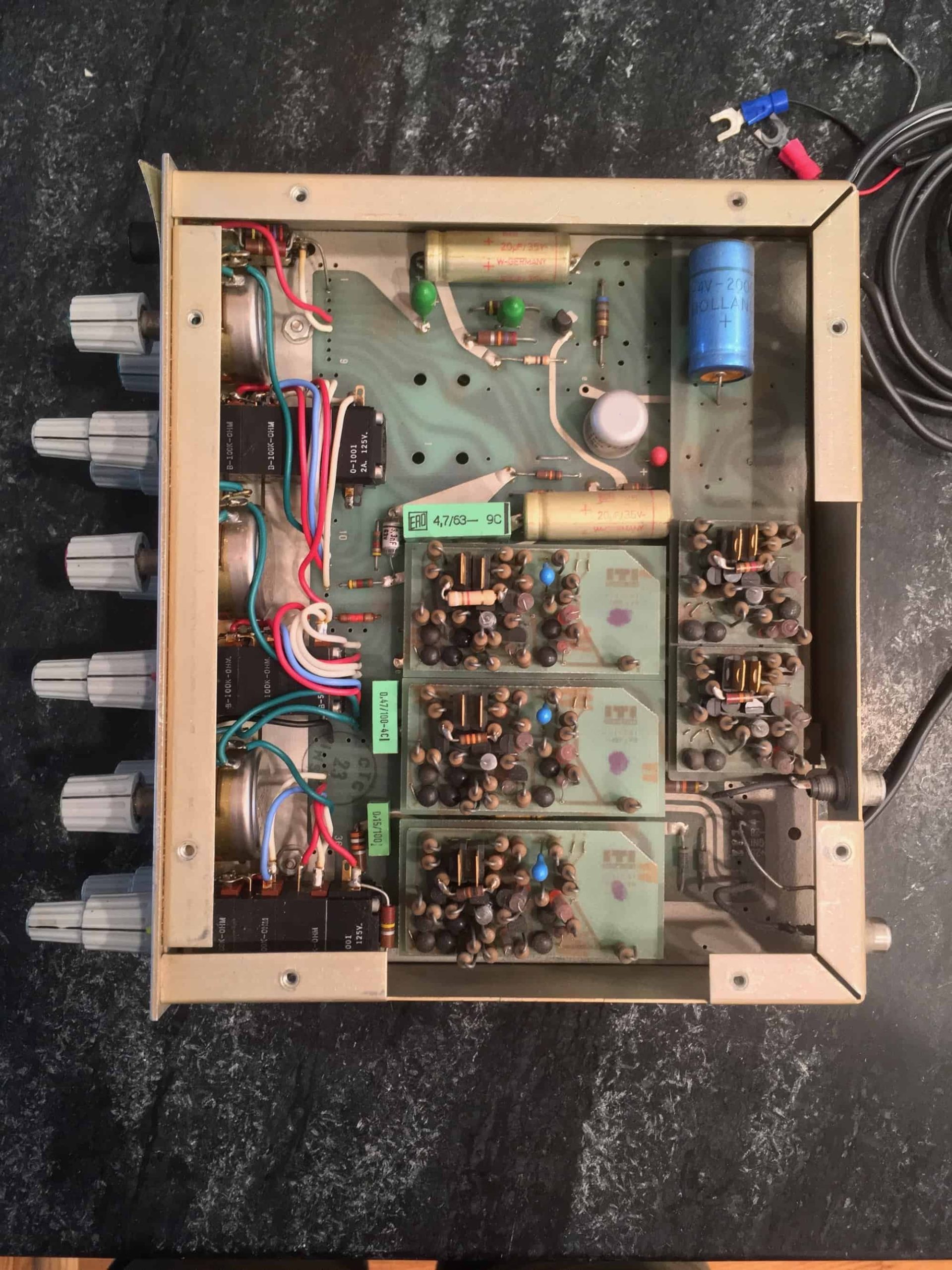
Inside an ITI MEP-130 module: the controls are along the left edge; the small circuit boards carry the filtering and amplification circuits.
Before 1972: inductors, capacitors and switches
Massenburg begins with a survey of the existing technology. For decades, tone correction had relied on a few families of passive circuits, collected in his Figure 1. A resistor–capacitor network, with a potentiometer controlling the depth, progressively reduces bass or treble (droop) or creates a step between two levels (shelf, what we now call shelving equalisation). A bell-shaped response requires a tuned inductor and capacitor, with a switch selecting the frequency from several inductor taps.

Figure 1 from George Massenburg’s paper (AES, 1972): the five traditional circuits. AI-assisted restoration of an archival document (original document). Each schematic is on the left and its frequency-response shape on the right; the VARIABLE arrow identifies the potentiometer’s adjustment. In 1E, the switch selects inductor tap F1, F2 or F3, hence the bell frequency.
These passive networks attenuate the signal, and an amplifier must restore the lost level. For domestic equipment, two bass and treble controls often suffice, as in the active Baxandall control discussed earlier. The studio L-C equalisers described here select frequencies by switching inductors and capacitors. This limitation applies to these switched-frequency networks: continuously tunable active prototypes already existed in the late 1960s.
The late 1960s: the operational amplifier enters the console
The first inexpensive hybrid and integrated circuits brought a new kind of console, including those from Data-Mix and Electrodyne. Massenburg criticises their still-immature technology but praises their architecture, summarised in Figure 2A. A potentiometer sits between an operational amplifier’s two inputs: its upper end connects to the non-inverting input receiving the signal, its lower end to the inverting input receiving feedback (a portion of the output returned to the inverting input). Its wiper connects to ground through a resistor–capacitor–inductor branch tuned by the switch. At resonance, this branch behaves almost like a short circuit. Towards DIP, it shunts the input signal and creates a dip; towards PEAK, it shunts the feedback, increasing amplifier gain and producing a bell. At the midpoint, marked “0”, the two effects balance and the response remains flat.

Figure 2A from George Massenburg’s paper (AES, 1972), “Feedback L-C Equalizer (Peak and Dip)”. AI-assisted restoration of an archival document (original document). Junction dots, absent from the original, have been added; the dot at the crossing below the second potentiometer indicates that this wire belongs to the same node as the bottom of the first potentiometer: the inverting input.
The circuit has no insertion loss, uses fewer components, and already lends itself to automatic control: a simple potentiometer or switched resistor ladder moves from peak to dip. But it retains its switches and inductors. Adding more potentiometers between the same two inputs produces a graphic equaliser, one band per slider (Figure 2B).

Figure 2B from George Massenburg’s paper (AES, 1972), “Feedback L-C Graphic Equalizer (Multiple Peak)”. AI-assisted restoration of an archival document (original document). Each band adds a potentiometer between the two inputs and its own resistor–capacitor–inductor branch; the dashed band N indicates that further bands can be added.
Massenburg immediately identifies the limitation described at the beginning of this chapter: more bands mean more sliders, narrower bells, longer adjustment times and bulkier equipment. Large models cannot fit into every console channel, while small ones remain just as slow to adjust.
The 1972 design requirements
Massenburg was writing as multitrack recording became established, and he looked further ahead. He believed the day was approaching when sound would be converted into digital words on entering the studio, processed and mixed in that form, and converted back only for listening. This was ten years before the compact disc. Every device would therefore eventually need to communicate with memory and a computer, and the project set three objectives:
- Automation: every function previously adjusted by a switch should be controllable by a simple variable resistor or a variable-gain stage;
- Eliminating inductors: heavy and imprecise, they pick up mains hum, while their parasitic capacitance causes unwanted resonances; transformers, Massenburg notes, were also disappearing from modern equipment;
- Unprecedented flexibility: giving the sound engineer complete control over every adjustment.
The requirements followed. Frequency, peak or dip amplitude, and response shape would all be continuously adjustable. The module would fit into a console channel without crowding its controls. Three \pm 12\ \text{dB} bands would overlap widely, spanning below 20\ \text{Hz} to above 20\ \text{kHz}. Dynamic range, noise and bandwidth would meet the state of the art, phase response would improve, and unwanted effects would be minimised. Inductors and transformers were therefore ruled out.
The first inductor substitute: the gyrator
The most direct solution has a familiar name: the gyrator, an active circuit whose input presents an impedance proportional to the inverse of the impedance connected at its output (impedance is frequency-dependent opposition to current). Loaded with a capacitor, it looks like an inductor from its input. Massenburg gives the simplest two-amplifier version in Figure 3.

Figure 3 from George Massenburg’s paper (AES, 1972), “Simple Gyrator”. AI-assisted restoration of an archival document (original document). A capacitor connected at Z_L produces an apparent inductance at Z_{IN} in the gyrator model. This is a historical functional schematic: amplifier characteristics are not specified, and the two triangles do not constitute a circuit that can be wired directly using two ordinary op amps.
Its advantages are those seen with the graphic equaliser: less parasitic capacitance, hence fewer unwanted oscillations, and much less hum pickup, even without shielding. But the circuit is difficult to set up and may cost more than a real inductor. Massenburg retains it only as an option in the bass shelving circuit.
The heart of the invention: turning a dip into a peak
For bell responses, Massenburg takes another route: the bridged-T filter (Figure 4). Two series resistors R form a T with capacitor C_2 running down to ground, while capacitor C_1 bridges the top. At low frequencies, the signal passes through the resistors; at high frequencies, through C_1; between them, the two paths almost cancel and the response falls into a dip. This is a notch filter, which rejects a narrow frequency band, with its minimum at:
Changing both resistors together, using a dual-gang potentiometer whose tracks follow each other accurately, therefore sweeps the frequency without changing the shape: f_0 varies inversely with R. The bridged-T never quite cancels the signal, however. At the bottom of the dip, it passes the fraction:
The larger C_2 is relative to C_1, the deeper the dip: with C_2 two hundred and fifty times larger than C_1, it reaches -42\ \text{dB}.

Figure 4 from George Massenburg’s paper (AES, 1972), “Basic Notch”. AI-assisted restoration of an archival document (original document). The bridged-T and its response shape: widely flared sides and a very narrow bottom.
Then comes the key idea. Invert this dip and it becomes a peak exceeding 40\ \text{dB} (Figure 5), far too high and narrow to use directly, but with a frequency that can be swept using a single dual-gang potentiometer.

Figure 5 from George Massenburg’s paper (AES, 1972), “Inverted Notch”. AI-assisted restoration of an archival document (original document). The inverted dip from Figure 4, before shaping: more than 40 dB from baseline to peak.
To invert the dip, the bridged-T is placed in an amplifier’s feedback loop, between the output and inverting input (Figure 6). The signal enters the non-inverting input, and circuit gain is the inverse of the T network’s transmission. At the notch frequency, the T returns almost nothing to the inverting input: deprived of feedback, the amplifier’s gain rises sharply.

Figure 6 from George Massenburg’s paper (AES, 1972), “Peak Inversion”. AI-assisted restoration of an archival document (original document). The bridged-T, enclosed by a dashed box, connects the output to the inverting input.
The peak must now be tamed. Massenburg adds a shape control to the amplifier loop, adjusting both peak height and the section’s input level. The two effects compensate at the summit: turning the knob leaves the bell’s height unchanged while its sides spread or narrow. This provides continuous adjustment of the quality factor Q, the bell’s selectivity.
Moving the level control outside the resonator
The section now has three parts—an input, an output and the processor between them—and can no longer be connected like the L-C branch of Figure 2A. Massenburg connects it as shown in Figure 8. This is not a four-amplifier state-variable filter: each band contains a bridged-T section and its shaping amplifier, with an output amplifier performing the summation.

Figure 8 from George Massenburg’s paper (AES, 1972), “Basic Parametric Section”. AI-assisted restoration of an archival document (original document). The rectangular block contains the tunable bridged-T in the peak-shaping amplifier’s loop; the processing and output amplifier performs the summation.
The level control is the PEAK / DIP potentiometer. One end of its track receives the system input (PEAK side), the other its output (DIP side), and a centre tap connects to ground. Its wiper feeds the shaping section, whose output is added to the direct signal at the output amplifier. Three positions explain the circuit:
- At the midpoint, the wiper sits on the grounded tap. The section receives no signal and adds nothing: the response is flat at 0\ \text{dB}.
- Towards PEAK, the wiper takes an increasing fraction of the input signal. The section adds its bell to the direct signal, boosting the band.
- Towards DIP, it takes a fraction of the output signal. The section is now in the output amplifier’s feedback loop, and its bell becomes a dip, attenuating the band. Massenburg emphasises that the control takes the equaliser from a bell response to its exact inverse.
Grounding the centre tap guarantees a zero signal at the midpoint. Without it, the centred wiper would receive the average of input and output. That average cancels only if the output stage inverts the signal exactly and both halves of the track are precisely equal, two conditions that real components never meet perfectly.
Crucially, this control acts outside the resonant circuit: turning the level knob does not change the resonator setting. The convention used to measure the complete correction’s bandwidth must still be specified, since the response also contains the direct signal. Figure 7 shows the correction at three levels, +12, +6 and +2\ \text{dB}, for two shape settings. The historical annotations of 4 and 9\ \text{dB} per octave describe the local slopes, not asymptotic slopes: far from the centre, all these bells return to 0\ \text{dB}. The redrawn curves are calculated and fitted to readings from the document; they are not new measurements of the hardware.

Figure 7 from George Massenburg’s paper (AES, 1972), “Peak ‘Q’ versus rotation of AMPLITUDE”. AI-assisted restoration of an archival document (original document). Three levels for two shape-control positions; the dB/octave figures are local indications from the historical document.
Figure 9 shows the other control: four shape settings, in both boost and cut, with the peak remaining close to \pm 12\ \text{dB} as the sides spread.

Figure 9 from George Massenburg’s paper (AES, 1972), “‘Q’ versus rotation of SHAPE”. AI-assisted restoration of an archival document (original document). The control mainly changes bandwidth, with the peak staying near \pm12\ \text{dB}. The calculated curves are fitted to historical readings whose peaks are not all exactly identical.
The complete system: two shelves and three bells
Figure 10 brings everything together. Three parametric sections, LOW, MID and HIGH, share the same output amplifier, and their three centre taps share a ground connection on the left of the schematic. At the front, a shelving section makes the device a complete programme equaliser. It follows the principle of Figure 2A: two potentiometers between an amplifier’s inputs. The first wiper connects to ground through a resistor and capacitor acting only at high frequencies: the treble shelf. The second passes through the gyrator, the inductor without a coil, acting only at low frequencies: the bass shelf.

Figure 10 from George Massenburg’s paper (AES, 1972), “Full System”. AI-assisted restoration of an archival document (original document). Left: the shelving section and its gyrator. Right: three sections as in Figure 8, with a potentiometer between input and output buses, grounded centre tap, wiper feeding the bridged-T and its amplifier, and summation at the output amplifier. The crossing below the shelving section’s second potentiometer has a junction dot, absent from the original.
Figure 11 gives the resulting shelves in boost and cut: two bass shelves reaching half their effect around 70\ \text{Hz} and 140\ \text{Hz}, and a treble shelf around 7\ \text{kHz}. Massenburg adds “active transformers” at the input and output: low-gain amplifiers that, like transformers, reject signals common to both wires of a balanced line and tolerate one wire being shorted without changing level.

Figure 11 from George Massenburg’s paper (AES, 1972), “Shelving Curves”. AI-assisted restoration of an archival document (original document). The bass and treble shelves are close to \pm12\ \text{dB}; the curves are recalculated and fitted to historical readings. The topology aims for reciprocal boost and cut responses, but these readings do not establish perfect reciprocity in the actual hardware.
“Blue skies”: automation as imagined in 1972
Massenburg closes with a section titled “Blue Skies Department”, devoted to future possibilities. He proposes replacing adjustable resistors with resistors switched by field-effect transistors (voltage-controlled electronic switches), driven by a six-bit word. In Figure 12, the six branches with values 32R, 16R, 8R, 4R, 2R and R are in parallel. For ideal switches, their conductances (the reciprocals of resistance) add: G=\sum_i b_i/R_i, where b_i is 1 for a closed branch and 0 otherwise. The 64 states therefore provide uniform conductance steps, with 63 finite equivalent resistances and one open circuit; resistance R_{\mathrm{eq}}=1/G does not change in uniform steps. Each bit is held by a D flip-flop (a one-bit memory copying its D input on each clock pulse), then conditioned by a small two-transistor stage repeated on each line.

Figure 12 from George Massenburg’s paper (AES, 1972). AI-assisted restoration of an archival document (original document). The MSB and LSB labels are retained from the original, but their order is reversed relative to conductance weights: the R branch contributes thirty-two times as much as the 32R branch. The scan ends before the caption; only Δ remains legible on the right-hand arrow.
In this proposal, a central analogue-to-digital converter reads the front-panel potentiometers in sequence. Their positions can be stored and then sent back to the corresponding functions. The resistor network is digitally controlled without a separate digital-to-analogue converter for each adjustment; the control law must nevertheless be adapted to the desired quantity. Six bits alone guarantee neither uniform resistance steps nor uniform frequency or gain steps.
Massenburg’s conclusions
For Massenburg, the parametric equaliser was a successful compromise between the three-knob switched-frequency equaliser, the graphic equaliser and the programme equaliser, with automation added. It can create a very narrow rejection notch and maintain it at different depths, for example to remove the bass resonance of an acoustic guitar recorded with a cardioid microphone. At its widest setting, its bell is broader than those of most equalisers. Above all, it is fast: sweeping the frequency lets the engineer hear the bell pass over the problem and immediately judge where and how much to correct. The mid band can broadly lift the upper midrange while the high band cuts vocal sibilance concentrated at one frequency. It can imitate loudness-compensation curves, while frequency sweeping opens the door to special effects. Massenburg saw it as a first step towards complete control of the spectrum and a foundation for future automation.
From the ITI MEP-130 to celebrated consoles: Neve, SSL, Trident and GML
ITI marketed this family as the MEP-130 channel module and ME-230 stereo rack unit, the latter having been presented in 1971 according to Massenburg. The MEP-130 technical manual, in the copy accompanied by 1976 test reports, describes three overlapping bands (10\text{–}800\ \text{Hz}, 100\text{–}8\ 000\ \text{Hz}, 400\text{–}25\ 600\ \text{Hz}) and continuously variable correction shape. In a May 1973 advertisement in db – The Sound Engineering Magazine, ITI highlighted continuous frequency, gain and shape controls.
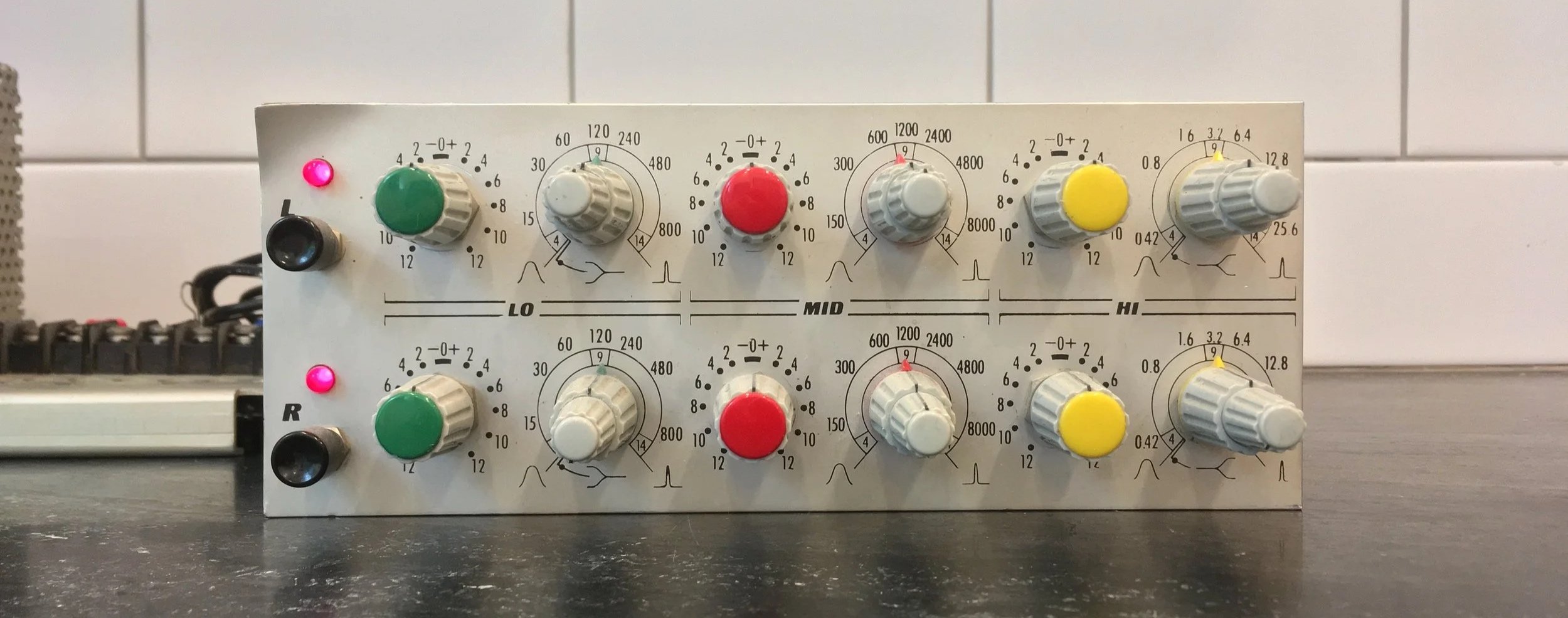
Two ITI MEP-130 modules housed together: the upper row processes the left channel (L), the lower row the right channel (R). In each row, LO, MID and HI identify the low, mid and high bands. The coloured knobs adjust gain from -12 to +12\ \text{dB}; to their right, two concentric knobs on a shared shaft adjust frequency and selectivity (the width of the correction). The small bell-shaped symbols indicate broad or narrow correction.
Around the same time and in subsequent years, console manufacturers developed various forms of adjustable equalisation; this chronology does not demonstrate a direct lineage from ITI. The Neve 1081, introduced in 1972, offered switched frequencies and a “Hi-Q” option on both mid bands. Trident developed the A-Range in 1971, followed by the Series 80 in 1980. Solid State Logic’s SL 4000 E, launched in 1979, had four bands including two parametric mid bands; the “02” or “Brown Knob” card was followed by the “242” or “Black Knob” card, developed in 1983. Massenburg founded GML (George Massenburg Labs) in 1982; its 8200 became a reference parametric equaliser for studio and mastering work.
Massenburg’s historical circuit is not the only way to provide these parameters. Section 5 will examine another particularly flexible structure, the KHN state-variable filter, followed by the limitations of the mixing network chosen for this article.
3. The three degrees of freedom of a parametric section
Parametric equalisation lets us choose where to act, over what bandwidth and by how much. The next figure illustrates a target model with three independent controls; it does not show the wiring of the KHN circuit studied later.

- Centre frequency f_0 moves the correction through the spectrum. In this model, changing f_0 preserves the centre gain and relative bandwidth, described by Q.
- Selectivity Q describes how narrow the correction is. Its bandwidth convention must be specified: in this figure, \Delta f is measured at half the gain in decibels, meaning +6\ \mathrm{dB} for a boost of +12\ \mathrm{dB}, or -6\ \mathrm{dB} for a cut of -12\ \mathrm{dB}. We then define Q=f_0/\Delta f. At zero gain, the response is flat and this bandwidth can no longer be read from the curve. For a pure band-pass, the usual convention instead measures bandwidth between the two points at -3\ \mathrm{dB} relative to the peak; it must not be transferred carelessly to a correction mixed with the direct signal.
- Centre gain sets the boost or cut. The three examples shown are -12, 0 and +12\ \mathrm{dB}. These are model settings, not a promised range for any potentiometer. A dedicated notch mode can provide ideal cancellation; its actual depth depends on matching and component limitations.
Using the figure’s bandwidth convention, the musical width is N=24\,\operatorname{asinh}(1/(2Q))/\ln 2 semitones. It is approximately 30.5 semitones for Q=0.5, 11.3 for Q=1.5, 3.46 for Q=5 and 1.73 for Q=10. It falls below half a semitone beyond Q\approx17.3. For Q=30, it is still 0.58 semitone: approximately Q=34.6 must be exceeded to fall below a quarter tone, or 0.5 semitone.
Control independence is a design objective that must be checked in the chosen circuit. Using op amps alone does not guarantee it. In the KHN circuit in Section 7, adjusting Q also changes the band-pass level and therefore the correction obtained by mixing; that section’s curves show this coupling using the actual component values.
4. Twin-T and Sallen–Key constraints when implementing three controls
Let us return briefly to the second-order sections introduced in Part Two. Why could we not simply fit three potentiometers to a twin-T filter or Sallen–Key section and obtain a parametric equaliser?
The twin-T difficulty: keeping three resistances tracking
Recall that a twin-T’s characteristic angular frequency is \omega_0 = \dfrac{1}{RC}. To vary f_0 continuously over a decade, for example from 100\ \text{Hz} to 1\ \text{kHz}, the passive network’s resistances must vary. But the twin-T requires two resistances of R and a third of exactly R/2.
Frequency can therefore be controlled with three jointly operated variable resistors, maintaining the ratio R:R:R/2. A triple-gang potentiometer (three tracks on one shaft) is one possibility, but its tracking must be checked: the resistance ratios must remain correct throughout the travel. The tolerance on total resistance does not guarantee this property.
Cancellation in a twin-T depends on balance between the network’s two branches. Mismatch can move the zero off the imaginary axis j\omega and limit notch depth. Consider a specific case: a nominal notch at 1\ \text{kHz}, an ideal source, an unloaded output, and the first series resistor from the input increased by +2\ \%, then by +20\ \%, with the other five components at nominal values. Searching for the new minimum each time, the passive twin-T (Q=0.25) gives approximately -58 and -40\ \text{dB}. With ideal bootstrapping (the network’s lower node receives k=0.95 times the output, giving nominal Q=5), these minima become approximately -32 and -12\ \text{dB}, shifting to 993 and 933\ \text{Hz}. These are results for this example, not universal limits for any 2\ \% error: changing another component or measuring at the nominal frequency produces different values. Continuous tuning remains possible, but maintaining a narrow, deep notch requires excellent tracking of the three resistors.
Sallen–Key: separating frequency tuning from gain/selectivity coupling
In Sallen–Key low-pass and high-pass sections, quality factor Q depends on resistance and capacitance ratios and on internal gain K. With two equal resistors and two equal capacitors, the natural frequency is f_0=1/(2\pi RC) and the quality factor simplifies to:
Varying both resistors by the same ratio therefore changes f_0 without changing Q: frequency adjustment is not inherently coupled to damping. However, adjusting Q through K also changes section gain. As K approaches 3 from below, sensitivity to tolerances increases sharply. In the ideal model, K=3 eliminates damping; K>3 produces an unstable system. A high but finite Q therefore does not by itself imply spontaneous oscillation. Sallen–Key band-pass sections have different equations, but also exhibit gain/selectivity coupling. An additional network or a different architecture is needed to obtain the three desired controls.
Another approach distributes the coefficients among several active blocks: two integrators for frequency, a feedback path for damping, and an output summation. This is the state-variable filter principle.
5. A flexible architecture: the state-variable filter (KHN)
In 1967, W. J. Kerwin, L. P. Huelsman and R. W. Newcomb published a state-variable filter synthesis. The KHN structure, named from their initials, appears notably in the Burr-Brown / Texas Instruments UAF42 integrated circuit and in Analog Devices examples. It provides simultaneous high-pass, band-pass and low-pass outputs, making it one useful option among several equaliser architectures.
The principle: implementing a differential equation with pure integrators
Instead of cascading passive filters, the state-variable filter uses operational amplifiers to solve a second-order differential equation in real time: a relationship between voltage and its changes over time. For the low-pass output v_{LP} of the resistor network chosen here, the input factor is K=1-1/(2Q):
The first two terms describe respectively the acceleration and rate of change of voltage; the last term on the left depends on voltage itself. Factor K sets the input signal’s weight. A normalised equation with K=1 describes the same type of response, but not this network’s exact gain.
To solve this equation, the structure uses two cascaded inverting integrators (to integrate means to accumulate over time), fed back to a summing stage. It avoids directly implementing differentiation (to differentiate means to measure the instantaneous rate of change), which strongly boosts high-frequency noise and requires suitable bandwidth limitation. Each integrator capacitor has impedance Z_C=1/(jC\omega):

Sign distribution and stability of the ideal model
In the network below, adapted from the KHN principle documented by TI for the UAF42, the labels and values are those used in this article:
Both integrators A2 and A3 are inverting:
V_{BP} = -\,\frac{\omega_0}{s}\,V_{HP} \qquad \text{and} \qquad V_{LP} = -\,\frac{\omega_0}{s}\,V_{BP} = +\,\frac{\omega_0^2}{s^2}\,V_{HP}Input summing amplifier A1 uses both inputs (V_- and V_+) to distribute the polarities:
The inverting input V_- receives feedback V_{HP} through R_1 = 10\ \text{k}\Omega and feedback V_{LP} through R_2 = 10\ \text{k}\Omega:
v_- = \frac{V_{HP} + V_{LP}}{2}- The non-inverting input V_+ receives input signal V_{in} through R_{in} = 10\ \text{k}\Omega, the ground reference through R_G = 10\ \text{k}\Omega, and band-pass feedback V_{BP} through selectivity resistor R_Q = R_{Q0} + P_2.
The voltage at this input is a weighted average, not a direct sum:
v_+=\frac{G_{in}V_{in}+G_QV_{BP}}{G_{in}+G_G+G_Q},\qquad G_{in}=\frac{1}{R_{in}},\quad G_G=\frac{1}{R_G},\quad G_Q=\frac{1}{R_Q}.Each G is a conductance, the reciprocal of resistance: a smaller resistor gives greater weight to the voltage it connects.
Setting v_- = v_+ under ideal linear operation gives V_{HP}=KV_{in}+V_{BP}/Q-V_{LP}. With the two inverting integrators, the characteristic equation is:
s^2 + \left(\frac{2\,G_Q}{G_{in} + G_Q + G_G}\right)\omega_0\,s + \omega_0^2 = s^2 + \frac{\omega_0}{Q}\,s + \omega_0^2The coefficients are positive for Q>0 and \omega_0>0: the ideal second-order model is stable. This does not guarantee stability of the real circuit, which also depends on the op amps’ frequency limitations and their layout. The quality factor, which controls selectivity, is:
Q = 0.5 + \frac{R_{Q0} + P_2}{10\ \text{k}\Omega}With a fixed series resistor R_{Q0} = 2.1\ \text{k}\Omega and a linear potentiometer P_2 = 100\ \text{k}\Omega, Q varies continuously and progressively from Q_{min}=0.71 (close to the Butterworth value 1/\sqrt{2}\approx0.707) to Q_{max}=10.71 (a narrower band).
Protecting the integrators: the essential fixed series resistors R_{min}
In a physical circuit, the input resistance of integrators A2 and A3 must never approach 0\ \Omega when potentiometer P_1 reaches an end stop:
- If input resistance vanished, natural angular frequency \omega_0 = \dfrac{1}{R_f C} would tend theoretically to infinity;
- The preceding op amp would have to supply excessive current into the integrator’s virtual ground (an input held near 0 V by feedback). Depending on the op amp and signal amplitude, current limiting or saturation would invalidate the intended operation.
To constrain the adjustment range safely, two identical fixed resistors R_{min} = 1.6\ \text{k}\Omega are placed in series, one with each track of dual-gang potentiometer P_1 = 100\ \text{k}\Omega:
- At minimum resistance (P_1 = 0\ \Omega), input resistance is exactly R_{min} = 1.6\ \text{k}\Omega, bounding the maximum frequency at f_{max} = \dfrac{1}{2\pi \times 1600 \times 10^{-8}} \approx 9.95\ \text{kHz}.
- At maximum resistance (P_1 = 100\ \text{k}\Omega), total resistance is 101.6\ \text{k}\Omega, setting the minimum frequency at f_{min} \approx 157\ \text{Hz}.
These resistors bound the nominal range to approximately 157\ \text{Hz}–9.95\ \text{kHz} and prevent zero input resistance. They do not guarantee freedom from saturation: signal amplitude must also be limited, allowing for band-pass gain, which increases with Q. Both tracks of P_1, and the track of P_2, are used as rheostats (two-terminal adjustable resistors), with each wiper connected to one end of its track.
Creating an ideal notch by summation
How do we obtain a notch filter from this circuit? In the twin-T, cancellation requires balance between the resistive and capacitive branches. In a state-variable filter, a transmission zero can be obtained by adding the high-pass and low-pass outputs in a summing amplifier.
For the actual network described (R_{in}=R_G=R_1=R_2=10\ \text{k}\Omega), the transfer functions (output-to-input voltage ratios) contain a common factor K=1-1/(2Q). Branch R_Q loads the non-inverting input: unity gain cannot be assumed for every setting of Q. They are:
Adding these two voltages (V_{notch} = -(V_{HP} + V_{LP})) gives the overall transfer function:
Consider the numerator at the resonant angular frequency p = j\omega_0:
The numerator cancels exactly and mathematically in this ideal model with identical integrators. In this model, two equal summing resistors (R_N = 10\ \text{k}\Omega) give the high-pass and low-pass outputs equal weight. These outputs remain exactly opposite in phase at every frequency. With ideal op amps, a mismatch between the two summing resistors or between the two integrators therefore only shifts the cancellation frequency: the weighted sum still cancels at a nearby frequency. In a real circuit, op-amp and capacitor imperfections are the main limits on the achievable depth.

Four-op-amp principle schematic: A1 distributes feedback polarities; A2 and A3 are inverting integrators; A4 performs mixing or notch summation. SW1 has three ganged changeover contacts, shown in position M (mixing); position N implements the notch. Vin, VHP, VBP and VLP identify the same connections in both halves of the drawing. The mixing network does not guarantee \pm 15\ \text{dB} independent of Q (Section 7). Power supplies and decoupling capacitors are omitted: this principle schematic is not a complete construction plan.

Responses calculated from the specified resistor network, assuming ideal op amps without saturation. Left: varying f_0 at Q=3 and position u=0 of P_3. Centre: varying Q at a fixed P_3 position, showing that gain changes too. Right: several P_3 positions and notch mode. The exact frequency f_0 is included in the calculation; the ideal notch zero is clipped at the graph’s -50\ \text{dB} floor, without implying any achievable real depth. The relationship \Delta f=f_0/Q between the two points at -3\ \text{dB} relative to the peak characterises the band-pass alone; it does not apply directly to the mixed signal’s bell response.
6. An alternative architecture: the Bainter notch filter
The KHN state-variable filter requires three to four operational amplifiers per section. In 1975, engineer J. R. Bainter published another three-op-amp active structure in Electronics that deserves mention: the Bainter notch filter.
Bainter’s circuit combines simple blocks with two feedback loops. Notch depth is relatively insensitive to passive-component drift; its actual limit depends notably on amplifier gain and frequency response. The cancellation frequency, however, can shift. The circuit allows frequency and quality factor Q (which describes selectivity) to be adjusted with little interaction, without guaranteeing perfect immunity to temperature or ageing in the real circuit.
7. From a pure notch to mixing: checking what P₃ actually does
Adding a fraction of the band-pass signal to the direct signal changes a frequency band. But two opposite-polarity connections do not guarantee symmetrical adjustment in decibels. Let us check the proposed network using its actual resistors instead of assuming a range of \pm 15\ \text{dB}.

The figure shows the same op amp A4 in two configurations, not two additional amplifiers. In mixing mode, the wiper of P_3=10\ \text{k}\Omega receives V_{BP}. Let u be its position, between 0 and 1: u=0 corresponds to the end connected to the non-inverting input. The resistances between the wiper and the two inputs are then a=R_s+uP_3 towards V_+ and b=R_s+(1-u)P_3 towards V_-, with R_s=2.2\ \text{k}\Omega. Each comprises a fixed resistor and a portion of the same potentiometer track.
The direct signal reaches V_- through R_0=10\ \text{k}\Omega. The feedback resistor (the return path regulating gain) is also 10\ \text{k}\Omega, and R_g=5\ \text{k}\Omega connects V_+ to ground. Assuming an ideal op amp operating without saturation, summing the currents gives:
This formula includes all three branches reaching the inverting input, including the branch from P_3. At the mechanical midpoint, a=b=7.2\ \text{k}\Omega and m=0: the band-pass contributions cancel. What remains is V_{out}=-V_{in}, a magnitude of 0\ \text{dB} with signal inversion.
At the end stops, however, the result is not symmetrical. At its centre frequency, the section described above gives V_{BP}/V_{in}=-(Q-0.5). For Q=3, we obtain +11.70\ \text{dB} at u=0 and +14.97\ \text{dB} at u=1. Moving from the centre towards u=1, the magnitude first falls to cancellation, then rises again with opposite polarity. The end one might be tempted to label “Cut” is therefore not maximum attenuation. Gain also varies when P_2 changes Q: this network does not provide the three independent controls expected of a fully developed parametric equaliser.
Notch mode remains possible, but requires complete switching. A three-pole double-throw switch (three electrical selections operated by the same lever, or 3PDT) implements the two configurations shown:
- The first pole selects V_{in} or V_{HP} at the input of R_0, which becomes the first summing resistor R_{N1} in notch mode.
- The second connects the inverting input either to branch b or to V_{LP} through a second, separate resistor R_{N2}=10\ \text{k}\Omega.
- The third connects the non-inverting input either to branch a or directly to ground. R_g can remain connected: it is then shorted by the ground connection.
In notch mode, the direct signal and both branches of P_3 therefore cease to act on A4. Its two summing resistors and feedback resistor are all 10\ \text{k}\Omega, giving V_{out}=-(V_{HP}+V_{LP}). The high-pass and low-pass outputs are never connected directly together. This is the principle documented by TI; the preceding mixing network is a proposal in this article, not a symmetrical equaliser circuit validated by that source.
At f_0, the two ideal contributions cancel. Far from the notch, the magnitude gain tends towards K=1-1/(2Q), not necessarily 1: at Q=3, this represents -1.58\ \text{dB}. Actual notch depth depends notably on tolerances and op-amp limitations; the ideal model’s zero does not guarantee measured rejection of 45\ \text{dB}.
Comparing notch-filter and equaliser architectures
| Feature | Passive twin-T | Active bootstrapped twin-T | Graphic equaliser (gyrators) | Parametric equaliser (KHN state-variable) |
|---|---|---|---|---|
| Continuous f_0 adjustment | Possible with three ganged, well-matched resistances | Possible, but tracking is critical for a deep notch | Not provided in the fixed-frequency graphic equaliser described here | Yes (dual-gang potentiometer P_1 with fixed series resistors R_{min}) |
| Continuous Q adjustment | No (fixed at 0.25) | Yes (potentiometer adjusting k) | No independent control; bandwidth may vary with gain | Yes, independently (single potentiometer P_2 with fixed series resistor R_{Q0}) |
| Gain adjustment (boost/cut) | No (attenuation only) | No (attenuation only) | Yes (one slider per band, with a range set by design) | Possible with a suitable network; the mixing circuit described here depends on Q and does not guarantee \pm 15\ \text{dB} (Section 7) |
| Tolerance sensitivity | Depends on component and error; Section 4 example: minimum near -58\ \text{dB} | Sensitivity increases with Q; same example at Q=5: minimum near -32\ \text{dB} | Frequency and shape shift | Ideal zero retained, but shifted by unequal summation or integrators; actual depth limited notably by op amps |
| Op amps per band | 0 (or 1 buffer) | 2 followers | 1 per gyrator (1/2 NE5532) | 4 op amps (quad TL074 or 2× NE5532) |
| Typical application | Fixed mains trap, 50\ \text{Hz} / 100\ \text{Hz} or 60\ \text{Hz} / 120\ \text{Hz} depending on the country | Precision fixed filter | Overall room equalisation | Studio consoles, mastering, precise audio correction |
Conclusion
We began with a record that sounded thin and harsh without equalisation. Its response had been altered during cutting, and a preamplifier applied the inverse correction. The networks studied in this part aim either for faithful overall reproduction or for a deliberate change serving measurement or listening.
- Paired filters alter the signal to pass through a medium, then aim to restore it. In the ideal FM pre-emphasis/de-emphasis and RIAA cutting/playback models, the normalised responses are inverses and their product is 1. With magnetic tape, the complete chain—recording, medium, head and playback electronics—aims for a flat response; the two electrical gains are not simply inverses. Noise added along the way receives only the processing downstream of where it appears.
- Equalisation filters make lasting changes: to compensate for a sensor, loudspeaker or room, or simply to please the ear. Tone controls, presence, rumble and scratch filters, loudness compensation and graphic equalisers belong to this family.
- Weighting filters shape the response to imitate the ear, so that a measuring instrument hears more like we do.
All these examples use the building blocks of the previous parts: first- and second-order sections, poles and zeros whose contributions add in decibels. Active feedback lets the Baxandall control avoid a passive network’s permanent loss; the gyrator replaces a coil with an active circuit. The graphic equaliser distributes correction over fixed frequencies. The parametric equaliser, developed in the late 1960s and presented under that name by Massenburg in 1972, adds control of the frequency and bandwidth of each correction.
Other, less common equalisers could also be included here. One example is the cutting filter, which applies the inverse RIAA curve to a record before any listener hears it. There are also crossover filters dividing a loudspeaker system into bands, and filters correcting a particular driver. This concludes our study of analogue filters, which has taken us from mathematical foundations to sophisticated audio implementations. Yet it has only opened the door a little: the world of audio filters is a broad one indeed.

Sources and background
- Main source of inspiration. “Les filtres passifs et actifs”, Part Four, “les exemples pratiques”, by Emmanuel Deret, Hobbytronic No. 14, March 1992, pp. 2–8. Emmanuel Deret was editor-in-chief and one of the principal contributors to this French electronics magazine of the early 1990s. Original issues can be consulted at abandonware-magazines.org.
Additional references
- Peter J. Baxandall, “Negative-Feedback Tone Control”, Wireless World, vol. 58, No. 10, October 1952, pp. 402–405.
- George Massenburg, “Parametric Equalization”, 42nd Convention of the Audio Engineering Society, Los Angeles, 2–5 May 1972, presentation K-2 (no preprint number), AES E-Library, document 16171.
- George Massenburg, “Did Massenburg Really Invent the Parametric EQ?”, autobiographical essay, no publication date stated.
- ITI (International Telecomm, Inc.), MEP-130 Parametric Equalizer Channel Module Technical Manual, copy accompanied by 1976 test reports, including the original unit schematic (Figure 6) and parts list.
- ITI, MEP-130 advertisement, db – The Sound Engineering Magazine, vol. 7, No. 5, May 1973, p. 16 (digitised issue).
- Mat Leffler-Schulman, “The History of My ITI Audio MEP-130 Parametric Mastering EQ Modules”, Mat Leffler-Schulman Mastering / Mobtown Studios; front-panel and internal-circuit photographs © Mat Leffler-Schulman.
- W. J. Kerwin, L. P. Huelsman, R. W. Newcomb, “State-variable synthesis for insensitive integrated circuit transfer functions”, IEEE Journal of Solid-State Circuits, vol. SC-2, No. 3, September 1967, pp. 87–92.
- Burr-Brown / Texas Instruments, UAF42 Universal Active Filter, SBFS002B, Figure 1 and gain equations: common output factor and dependence of band-pass gain on Q. Report SBFA002, Figure 10: summation of high-pass and low-pass through two separate resistors. These references support the section and notch configuration; the mixing network in Section 7 does not come from them.
- Texas Instruments, NE5534x Low-Noise Operational Amplifiers, datasheet SLOS070D, revised November 2014 (pin table, p. 3; Figure 10, Frequency Compensation and Offset-Voltage Nulling Circuit).
- J. R. Bainter, “Active Filter Has Stable Notch, and Response Can Be Regulated”, Electronics, 2 October 1975, pp. 115–117.
- Philips Semiconductors, Audio circuits using the NE5532/3/4, application note AN142, October 1984, revision 2, August 1988: Figure 1, p. 2 (redrawn equaliser section), and component table, p. 3; Figures 14, 15 and 17 for NAB, rumble and loudness preamplifiers. Designators follow the schematic and table: R8 is the potentiometer; the note’s introductory text incorrectly calls it R9.
- Hank Zumbahlen, Basic Linear Design, Chapter 8: “Analog Filters”, Analog Devices, 2007.
- Analog Devices, A Beginner’s Guide to Filter Topologies, Application Note AN-1762.
- Analog Devices, ADALM2000 Activity: Active Filters – Part 2 (State-Variable KHN and Tow-Thomas), StudentZone, July 2024.
- Signetics, Analog Applications, 1979: loudness (p. 36, Figure 3-42); maximum cutting velocity for RIAA preamplifiers (p. 209); bias trap and NAB playback (pp. 214 and 218).
- National Semiconductor, Audio/Radio Handbook, 1980: maximum cutting velocity and typical record modulation velocities.
- Tomlinson Holman, “Dynamic Range Requirements of Phono Preamplifiers”, Audio, July 1977: cutting limits below and above 800\text{ Hz}, and peaks measured on commercial records.
- Stanley P. Lipshitz, “On RIAA Equalization Networks”, Journal of the Audio Engineering Society, vol. 27, No. 6, June 1979, pp. 458–481.
- Douglas Self, Small Signal Audio Design, 3rd edition, Focal Press / Routledge, 2020.
- ITU-R Recommendation BS.450-3, “Transmission standards for FM sound broadcasting at VHF”.
- IEC 61672-1:2013, Electroacoustics — Sound level meters — Part 1: Specifications: analytical forms of A and C weighting.
- Harvey Fletcher and W. A. Munson, “Loudness, Its Definition, Measurement and Calculation”, Journal of the Acoustical Society of America, vol. 5, No. 2, October 1933, pp. 82–108.
- National Semiconductor, Audio Handbook, 1976: Section 2.12, tape preamplifiers (recording-head current and bias trap, Example 2.12.1; turn-on time, Equation 2.12.8); Section 2.14, passive tone controls (Figures 2.14.1–2.14.6, worked Example 2.14.1, pp. 2-40–2-43).
- Nakamichi, Technical Bulletin 2: Playback Equalization, undated: cassette playback time constants according to Philips, IEC and DIN.
- Revox, B77 MK III Stereo Tape Recorder, Technical Data: NAB and CCIR equalisation, signal-to-noise ratio.
- Walter G. Salm, “The Dolby System — How it Works”, Radio-Electronics, October 1969: hiss reduction by the first Dolby system.
- Ray M. Dolby and Stanley G. Cossette, Audio compressor, expander, and noise reduction circuits for consumer and semi-professional use, US Patent 5,185,806, published 9 February 1993: definitions of Dolby A bands and the Dolby B sliding band.
- Ray M. Dolby, “An Audio Noise Reduction System”, Journal of the Audio Engineering Society, vol. 15, No. 4, October 1967, pp. 383–388.
- Analog Devices, Op Amp Applications, Chapter 6, Figures 6-9–6-17: RIAA-network synthesis and trade-offs between topologies.
- Texas Instruments, Analysis of the Sallen-Key Architecture, SLOA024B, Sections 3.4 and 4.4: natural frequency and quality factor with equal components; Active Notch Filters, SLYT235: twin-T adjustment and tracking.
- Analog Devices, Bainter Notch Filter, MT-203, and Texas Instruments, Analog Applications Journal, first quarter 2015, p. 10: adjustments and practical limits of notch depth.
- AMS Neve, 1081 User Manual; SSL, Channel Strip Guide; Trident, manufacturer’s timeline; GML, history and 9500 with stepped controls.