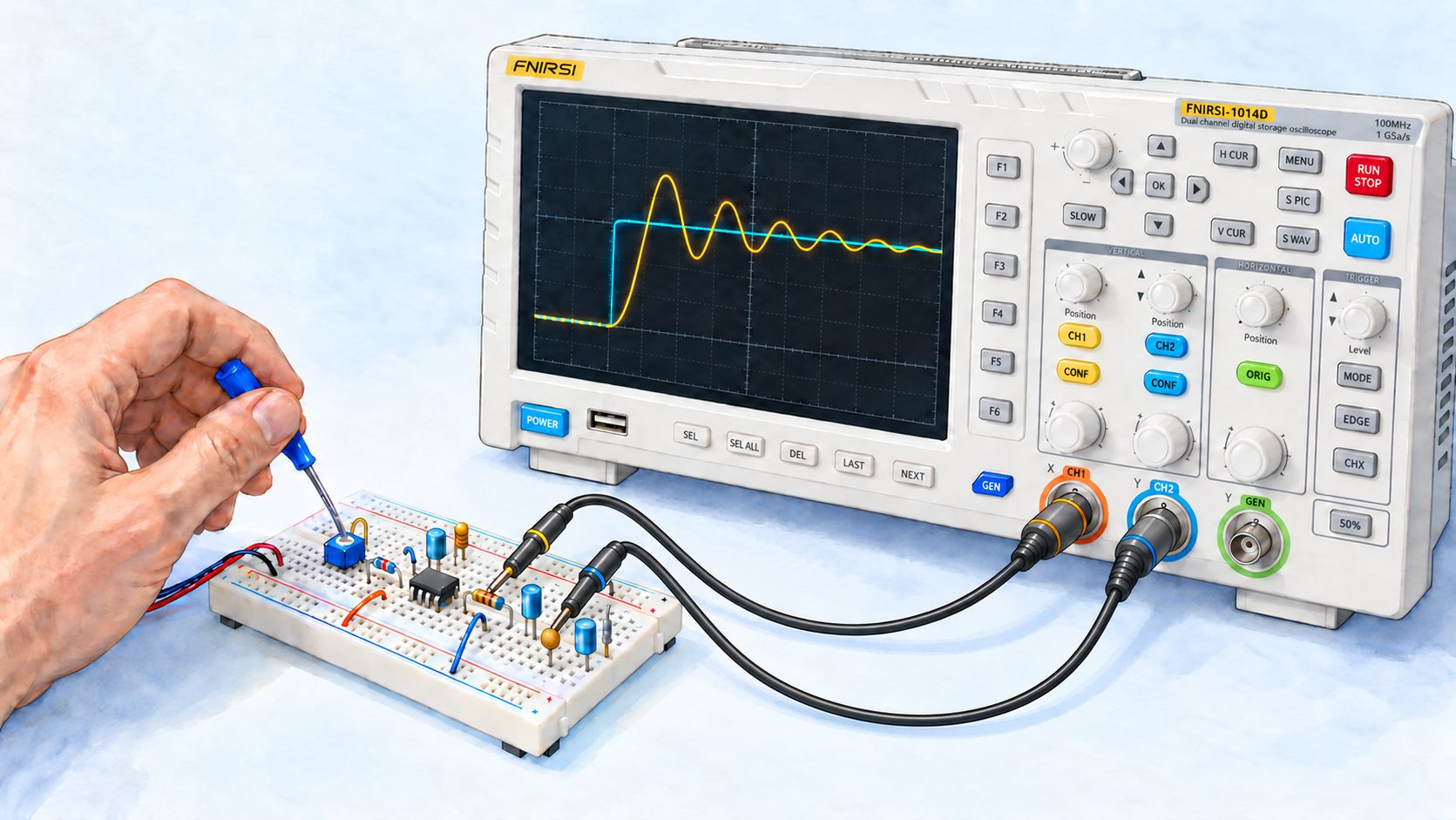
Take the operational-amplifier integrator that closed Part One and simply swap its resistor and capacitor. The resulting circuit is its exact mathematical mirror: it differentiates the input signal (measures how fast it changes from instant to instant) instead of integrating it. On paper, everything works. Build it, apply a square wave, and the oscilloscope will show a pulse followed by a long burst of damped ringing, at a frequency that appears in neither of the circuit’s two original formulas.
This ringing is not a wiring fault. We can calculate it, and that calculation alone explains why practical differentiators generally include additional limiting and stabilising components that elementary theory never asks for.
In Part One, we saw that a passive RC section cannot exceed a slope of -6\text{ dB} per octave, that two sections connected end to end load each other instead of simply adding their effects, and that a buffer solves this interaction without giving us control over the shape of the knee. We still need a way to control that shape. This instalment will provide it: we will see where the quality factor Q comes from in an active circuit, which architectures let us adjust it, and what each arrangement costs us.
In mathematics, integration always comes with its inverse, differentiation. Electronics is no different: the integrator has a counterpart, the differentiator, and its structure is exactly what we might expect—an integrator with its two components swapped. The capacitor moves to the input, and the resistor moves into the negative-feedback loop (the return path that feeds the output back to the inverting input and regulates the gain).
With an ideal operational amplifier, the inverting input is a virtual ground. The current through the capacitor is i = C\,\dfrac{\mathrm{d}V_I}{\mathrm{d}t}, and it has nowhere to go except through the feedback resistor. The output is therefore:
Here p is the Laplace variable, usually written s in English-language references; with zero initial conditions, multiplication by p represents differentiation (measuring the instantaneous rate of change). We retain p to match the original equations and diagrams.
This is indeed differentiation: the faster the input changes (the greater its instantaneous rate of change), the larger the output. On a Bode plot, the magnitude is a straight line with a slope of +6\text{ dB} per octave (+20\text{ dB} per decade), crossing 0\text{ dB} at the characteristic frequency f_d = \dfrac{1}{2\pi R C}.
On paper, this line rises indefinitely. In the physical circuit, however, the operational amplifier driving it does not have infinite gain. In open loop—the bare device, without any feedback components—its internal amplification \mu(p) is limited to a static value \mu_0 at DC, then inevitably falls beyond its internal cutoff \omega_c.
To understand why a real differentiator is so difficult to stabilise, we must put these two realities side by side. The comparison below shows both behaviours at three levels: circuit diagram, gain response and phase response.
Left column — Ideal differentiator (closed loop): the complete circuit with its feedback. Its gain demand rises indefinitely at +6\text{ dB} per octave (+20\text{ dB} per decade), while its phase remains exactly -90^\circ: the +90^\circ lead from differentiation combined with the 180^\circ inversion at the op amp’s inverting input.
Right column — Real op amp alone (open loop): the bare device, with no return path. Its available gain is limited to \mu_0 \approx 10^5 (100\text{ dB}), passes through the −3 dB point at its cutoff angular frequency \omega_c, then falls at -6\text{ dB} per octave towards the transition frequency \omega_T. Its phase starts at 0^\circ at DC, passes through -45^\circ at cutoff, and approaches -90^\circ at high frequency.
Fig. 1 — Comparison panel: the ideal closed-loop differentiator against the real op amp’s open-loop response
Why the rising slope always catches up with the amplifier
In the simplest first-order model, the op amp’s open-loop gain \mu behaves like a low-pass filter:
\mu(p) = \frac{\mu_0}{1 + \dfrac{p}{\omega_c}}
Here \mu_0 is the static gain (the gain at zero frequency, or DC—typically 10^5 to 10^6, or 100 to 120\text{ dB}), and \omega_c is the angular frequency of its dominant pole, often corresponding to only a few hertz. Beyond the −3 dB point set by \omega_c, the available gain falls at -6\text{ dB} per octave until it reaches unity at the transition frequencyf_T (the gain–bandwidth product listed in data sheets).
We are therefore faced with two opposing requirements that cannot negotiate with each other:
A gain demand that keeps rising at +6\text{ dB} per octave, because differentiating a high-frequency signal requires amplification proportional to its rate of change;
An amplifier’s available gain that runs out of steam and falls at -6\text{ dB} per octave, because its internal transistors cannot keep up indefinitely.
A rising line and a falling line will inevitably cross. The danger lies in how steeply they converge: their relative slope is (+6)-(-6)=12\text{ dB} per octave, or 40\text{ dB} per decade.
Fig. 2 — Rate of closure of 12 dB per octave: the critical crossing of gain supply and gain demand
In control engineering, this difference in slope is called the rate of closure. A closure rate of 12\text{ dB} per octave indicates that two first-order contributions are acting simultaneously here. The amplifier gain A contributes a lag tending towards -90^\circ, while the feedback factor \beta, whose reciprocal 1/|\beta| is the rising gain demand, also contributes a lag tending towards -90^\circ. The phase of the loop gain L=A\beta can therefore approach -180^\circ, leaving a dangerously small phase margin.
Stability is decided not by the graphical intersection alone, but by the phase of the loop gainL(p)=A(p)\,\beta(p) at the frequency where its magnitude reaches unity (|L|=1). The remaining angle before -180^\circ is the phase margin\varphi_m. With a comfortable margin, the circuit settles quietly; with a tiny margin, it rings strongly; as the margin tends to zero, it approaches marginal stability; with a negative margin, the loop is unstable.
Let us calculate it properly for our example. With feedback factor \beta(jf)=1/(1+jf/f_d), the loop gain reaches unity near 69.1\ \text{kHz} with a phase of -178.7^\circ, leaving a phase margin of just 1.3^\circ. It is not zero, but it is painfully small: the circuit is balanced on the edge of instability.
What the calculation really tells us: the real differentiator is a high-Q band-pass filter
Let us revisit the circuit with the amplifier’s finite gain included. Writing \omega_T=\mu_0\,\omega_c=2\pi f_T for the gain–bandwidth product, the exact transfer function becomes:
The denominator is a second-degree polynomial: the real differentiator is not a differentiator but a second-order band-pass filter, as its numerator in p confirms. Neglecting \omega_c compared with 1/RC—valid when the differentiator’s time constant is short compared with that of the amplifier’s dominant pole—and 1 compared with \mu_0, the result becomes clear:
In terms of frequency, with f_d=\dfrac{1}{2\pi RC} the differentiator’s characteristic frequency, where its gain is unity: ⚠️ this is not a natural frequency, since the ideal differentiator -RCp has no poles.
The first relation deserves a pause: the resonance frequency is the geometric mean of the differentiator’s characteristic frequency and the amplifier’s transition frequency. It belongs neither entirely to the external circuit nor entirely to the device: it emerges from their interaction. That is why neither original formula contains it when considered separately.
Take a concrete example: a TL071 (f_T=3\ \text{MHz}), R=10\ \text{k}\Omega and C=10\ \text{nF}. The differentiator’s characteristic frequency is f_d=1\,591.5\ \text{Hz}, and the calculation gives:
A quality factor of 43.4 corresponds to a damping ratio \xi=1/(2Q)\approx0.0116. Since the real differentiator is a band-pass filter with a zero at DC, its step response does not settle to a permanent plateau against which conventional overshoot could be defined. Instead, it produces damped ringing that returns to zero, with an envelope taking about 13.8 periods (Q/\pi) to fall to 1/e, and more than 41 periods to fall to 5\ \%. Exact numerical calculation of the complete response confirms the severity: a +65.4\ \text{dB} peak at 69.1\ \text{kHz}, reaching 32.7\ \text{dB} above the ideal +6\text{ dB}-per-octave asymptote.
Fig. 3 — Dynamic error of the differentiator: crossing slopes and a resonant peak at the geometric mean
Strictly speaking, the circuit is not a sustained oscillator—its poles remain in the left half-plane—but it is so close that a small additional parasitic capacitance may make it unstable. And its +6\text{ dB}-per-octave slope makes no distinction between useful signal and noise: it amplifies both with the same impartiality, concentrating them around 69.1\ \text{kHz}.
Damping the circuit: first a resistor, then a capacitor
The formula itself suggests the remedy. Since Q grows as \sqrt{RC}, and we cannot change RC without changing the intended function, we need an additional damping term. We therefore place a resistor R_1in series with the input capacitorC_1. It limits the gain demanded from the loop at high frequencies, while leaving low frequencies essentially unchanged, where the capacitor’s impedance (opposition to current that varies with frequency) dominates.
Keeping the approximation that the internal cutoff \omega_c is far below the circuit’s other angular frequencies, the gain–bandwidth product \omega_T=\mu_0\,\omega_c governs the second-order denominator. Here \mu_0 is the op amp’s static open-loop gain, its maximum DC amplification without feedback:
We obtain a Butterworth denominator: the response relative to the ideal differentiator is maximally flat (\xi=\sqrt{2}/2\approx0.707) for the ideal value:
For our example, the calculation gives R_1\approx325.7\ \Omega. Choosing the nearest E12 preferred value, R_1=330\ \Omega, gives an actual damping ratio \xi\approx0.716, very close to the theoretical 0.707. The original +65.4\ \text{dB} peak is shaved down to +29.5\ \text{dB}: the narrow spike disappears, although a broad maximum remains. The value R_2/R_1=30.3 describes an asymptotic plateau that would be well established if the two transition frequencies were sufficiently separated; they are not in this example. R_1 is our main damping adjustment. Since R_1\ll R_2, it has little effect on the natural frequency.
When the transitions are sufficiently far apart, we can identify three asymptotic regions:
Differentiator region, up to f_1=\dfrac{1}{2\pi R_1 C_1}\approx48.2\ \text{kHz}: slope +6\text{ dB} per octave; the circuit does its intended job.
Amplifier region, if an intermediate range exists: gain near R_2/R_1; the circuit is simply an ordinary inverting amplifier.
Integrator region, higher still: slope -6\text{ dB} per octave, once the demanded gain meets the amplifier’s available gain.
This is where the second component comes in. With R_1 alone, the third region is supplied by the amplifier pole—a manufacturing parameter that varies between devices, with temperature and with supply voltage. We would rather obtain it from a component we can choose: a capacitor C_2in parallel with the feedback resistorR_2. With the operational amplifier still assumed ideal, the transfer function becomes:
Fig. 4 — Differentiator stabilised by R1 and C2, and its three operating regions
The gain plot above (panel 2) shows both circuits together, revealing what C_2 changes. The grey dashed line is the response with R_1 alone, corresponding to the three regions just described; the solid blue line is the complete response we are about to obtain. Read its markers as follows:
At the top of the vertical axis, \mu_0 is the op amp’s static open-loop gain: its intrinsic DC amplification without feedback. The model used here is a typical TL071 with \mu_0=2\times10^5, or 106\ \text{dB}. This is the maximum amplification its internal transistors can provide. The pale dashed curve descending from it shows what remains available at each frequency.
The intermediate plateau R_2/R_1 is theoretically 29.6\ \text{dB}, a gain of 30.3. The grey curve peaks at 29.5\ \text{dB} because the op amp is already reducing it slightly.
Marker ③ shows where demanded gain meets available gain. ⚠️ The gain reached there is not \mu_0: \mu_0 is the DC gain, which the amplifier left behind at just a few hertz. Nor is the frequency calculated from signal gain R_2/R_1, but from noise gain1+R_2/R_1=31.3, the gain the feedback loop actually demands: f_T/(1+R_2/R_1)\approx96\ \text{kHz}. The difference is only 3\ \% here because the gain is high; for an inverting amplifier of unity signal gain, it would reach 100\ \%.
The phase plot (panel 3) shows the dynamic transition in the third-order model of the complete circuit, including the TL071’s dominant pole. ⚠️ The convention needs explaining: the physical transfer function V_O/V_I of an inverting circuit includes the minus sign, or static 180^\circ inversion, which would make the raw phase start at -180^\circ+90^\circ=-90^\circ. Here that static inversion has been removed to show only the filter’s dynamic behaviour: the phase lead from differentiation therefore starts at +90^\circ at low frequency. It crosses exactly 0^\circ at 39.1\ \text{kHz}, very close to the gain peak at 39.4\ \text{kHz}, marking the transition from differentiation (lead) to attenuation (lag). At higher frequencies, the op amp’s own pole adds to the network’s two poles, making the phase approach -180^\circ, a total dynamic excursion of 270^\circ. The displayed phase is unwrapped: continuous, without jumps modulo 360^\circ. The stabilising passive network alone would tend towards -90^\circ; the TL071’s dominant pole adds another 90^\circ of lag, giving the -180^\circ asymptote. In a wrapped display, -180^\circ is equivalent to +180^\circ, never +90^\circ. The continuous plot reveals the physical accumulation of these successive lags.
The usual choice R_1C_1=R_2C_2 puts both cutoffs at the same frequency; here, C_2=330\ \text{pF}. The blue curve shows the consequence: since both corrections act at the same frequency, there is no room for the plateau to form. The response goes directly from +6 to -6\text{ dB} per octave, rounding off at +23.6\ \text{dB} near 39\ \text{kHz}. That is 6\ \text{dB} below the maximum with R_1 alone, with much stronger attenuation beyond it.
⚠️ A word about damping: its value depends on the model being examined. With an ideal amplifier, setting R_1C_1=R_2C_2=\tau gives denominator (1+\tau p)^2: a double real pole, hence exactly \xi=1, with no resonance possible by construction. The real amplifier’s pole adds to these two and moves the dominant pair near 39.4\ \text{kHz}, with \xi\approx0.82. Both results are correct; they answer different questions. In either case, the circuit is well damped and its useful differentiation range remains intact up to a few kilohertz.
One wiring detail appears in the diagram: the non-inverting input is grounded through R_p\parallel C_p. At DC, R_p\approx R_2 can reduce the error caused by input bias currents if the two input currents are sufficiently similar. At AC, C_p lowers the input impedance and limits the thermal-noise contribution from R_p. This network does not guarantee equal impedances at both inputs over the entire band; its usefulness also depends on the op amp technology.
One final warning is needed, because references often omit it. These two components reduce the high-frequency gain demand and help stability; they do not guarantee it on their own. Phase margin must still be checked with the actual amplifier, output load and wiring. A few tens of picofarads of parasitic capacitance at the inverting input can change the conclusion.
Two variants using the same single amplifier
The differentiator above inverts the signal. Two rearrangements let us avoid this.
The differential differentiator places the same C–R network at both inputs. If R=R' and C=C', its output is proportional to the derivative of the difference between the two input voltages:
The non-inverting differentiator follows immediately: simply set V_{I1} to zero by connecting the corresponding input capacitor directly to ground. We then obtain V_O=+R\,C\,p\,V_I, without phase inversion.
Fig. 5 — Differential and non-inverting differentiators, in their ideal unstabilised form
⚠️ Both diagrams show ideal circuits. They inherit the problem established earlier in full: their +20\ \text{dB}-per-decade slope never stops by itself, so they face the same 12\ \text{dB}-per-octave closure against the amplifier curve and the same high-frequency noise amplification as the bare differentiator. In practice, a series resistor is added symmetrically to each input capacitor. When an extra capacitor provides the high-frequency limit, matched capacitors are placed across R and R'—the earlier stabilisation method applied to both branches. ⚠️ These additional components must be matched just like R, R', C and C': mismatch in the stabilising network degrades common-mode rejection just as mismatch in the main network does.
Before moving on, we should explain why this variant belongs in an article about filters: it adds a second selection criterion. Every circuit so far has selected signals by frequency, the defining job of a filter. This one still does: its slope is +6\text{ dB} per octave, exactly like the simple differentiator from which it comes. ⚠️ We should not call it a first-order high-pass filter in the usual sense: a first-order high-pass has a pole, hence a plateau beyond its cutoff, whereas the ideal differentiator R\,C\,p has none and rises indefinitely. It is a differentiator, behaving as a high-pass within its useful range—and that unbounded rise is precisely why we had to add a pole ourselves. It also selects according to how the signal appears on the two input wires: identical contributions are rejected, while differences are retained.
This second selection solves a problem that the first cannot touch. Frequency filtering cannot remove interference inside the useful passband: no order, no approximation, no eighth-order Butterworth can separate interference at 1\ \text{kHz} from a useful signal at 1\ \text{kHz}. If the interference instead reaches both conductors in the same way, as happens when an external disturbance couples sufficiently similarly into both, a differential arrangement rejects it without relying on frequency. This is why differential processing belongs at the front of a real signal chain: it removes what later filters cannot. ⚠️ That front end is normally a differential or instrumentation amplifier with flat gain. A differential differentiator belongs there only when the desired information is the rate of change of the difference. Its +20\ \text{dB}-per-decade slope amplifies high-frequency content, including noise, which is not what an ordinary input stage should do.
The formula deserves a closer look because it describes behaviour that intuition does not immediately supply. This circuit measures neither input signal individually: it measures how fast they move apart. Two perfectly identical voltages of several volts produce exactly zero output; two tiny voltages diverging quickly produce a clear output.
Take a target characteristic frequency of 10\ \text{kHz}. Unity gain occurs at f_d=1/(2\pi RC), requiring RC=15.9\ \mu\text{s}. With R=R'=16\ \text{k}\Omega and C=C'=1\ \text{nF}—available E24 and E6 values—we obtain RC=16\ \mu\text{s} and f_d=9\,947\ \text{Hz}, 0.53\ \% below target. Now apply two sine waves of identical frequency and amplitude, each 1\ \text{V} peak, and vary only their phase difference \varphi.
Two lines of calculation explain the entire figure. The difference between two equal-amplitude sine waves is itself a sine wave:
V_{I2} - V_{I1} = A\,[\sin(\omega t + \varphi) - \sin \omega t] = 2A\,\sin\frac{\varphi}{2}\,\cos\!\left(\omega t + \frac{\varphi}{2}\right)
Differentiating gives V_O=-2\,RC\,\omega\,A\,\sin\dfrac{\varphi}{2}\,\sin\!\left(\omega t+\dfrac{\varphi}{2}\right), so the output amplitude varies as \sin(\varphi/2)—and nothing else changes between the four panels. At \varphi=0, the inputs coincide, their difference is exactly zero, and the output remains flat despite two volts peak-to-peak at each input—provided the amplitudes also match. Zero phase difference means pure common mode only for equal amplitudes; an amplitude mismatch leaves a difference. At 45°, the output reaches 0.77\ \text{V}; at 90°, 1.42\ \text{V}; at 180°, the inputs differ as much as possible and the output reaches 2.01\ \text{V}. We move from exactly zero to 2.01\ \text{V} without changing either input’s amplitude or frequency.
This property, rather than differentiation itself, determines where the circuit is useful. Anything arriving identically at both inputs—called common mode, the part shared by both wires—takes the \varphi=0 route: it produces no output.
Two contributions that practice often conflates must be separated. The differential structure’s contribution, common-mode rejection, is useful in all the situations below. The differentiator’s addition, a +20\ \text{dB}-per-decade slope, is desirable only in the last.
Balanced transmission. When interference couples sufficiently similarly into both conductors, particularly through capacitive coupling or a shared electromagnetic environment, much of it appears as common mode and can be rejected by a differential input. The regular twist of a twisted pair also greatly reduces differential coupling, especially magnetic coupling, by alternating the polarity of exposed loops. The useful signal is carried by the difference between the wires and passes through intact. This is an application of a differential input, not differentiation: it uses a flat-gain balanced receiver, never a differentiator that would amplify high-frequency noise.
A strain-gauge bridge or a high-side current shunt. Both inputs sit at an unwanted high common potential. Again, the normal readout uses an instrumentation amplifier. Differentiation is appropriate only when the desired quantity is the rate of bridge imbalance—a shock, cracking event or pressure front—rather than the imbalance itself.
Edge detection on a transmission pair. This is the differential differentiator’s natural application: differentiating the difference produces a pulse at each transition, while a ground-potential difference between instruments, potentially several volts of pure common mode, produces nothing. The information is the rate of change, so differentiation is the measurement itself.
The conditions R=R' and C=C' are therefore not cosmetic: they ensure common-mode rejection. With an ideal op amp, a 1\ \% mismatch in one pair can limit external common-mode rejection to about 40\ \text{dB}, while the residual is amplified by the +6\text{ dB}-per-octave slope. ⚠️ This external limit must not make us forget the op amp itself: overall rejection combines passive-component matching with the amplifier’s intrinsic limits—its common-mode rejection ratio (CMRR) at the frequency of interest, bias asymmetries and falling loop gain. An excellent op amp CMRR cannot rescue passives matched to only 1\ \%, which is why 0.1\ \% resistors and selected capacitors are needed for high rejection. Conversely, a poor amplifier limits rejection even with ideal passives.
The integrator–differentiator: a band-pass filter with one amplifier
Since the damped integrator behaves as a low-pass and the damped differentiator as a high-pass, the next question follows naturally: what happens if we put both around the same amplifier?
Place a series C_1–R_1 network at the input and a resistor R_2 in parallel with capacitor C_2 in the feedback path. The output ratio is -Z_f/Z_i, with Z_i=R_1+\dfrac{1}{C_1p} and Z_f=\dfrac{R_2}{1+R_2C_2p}, giving:
This is exactly the stabilised differentiator’s transfer function. Changing its name has not changed the circuit: what we called stabilising a differentiator amounts to building a low-Q band-pass filter. This interpretation immediately gives its useful parameters:
Fig. 7 — The integrator–differentiator: a second-order band-pass with a single operational amplifier
This band-pass can never be very selective: its poles are real and distinct, or at best coincident, so Q\le0.5. It cannot isolate a narrow frequency range, but is valuable wherever one amplifier must reject DC at one end and high-frequency noise at the other—for example, to provide bandwidth-limited derivative action in a control loop. To exceed Q=0.5, the denominator must stop factoring into two real first-order terms. That is the subject of what follows.
Second-order active filters: the canonical form and what Q controls
A second-order active filter has a second-degree polynomial in its transfer-function denominator. We always write it in the same canonical form—a standard form separating gain, natural angular frequency and damping—so that two circuits sharing no components can be compared term by term:
\omega_0=2\pi f_0 is the undamped natural angular frequency;
\xi is the damping ratio;
Q=\dfrac{1}{2\xi} is the quality factor, also associated with voltage magnification in some resonant circuits.
Only the numerator N(p) distinguishes the four families: constant for low-pass, proportional to p^2 for high-pass, to p for band-pass, and to 1+p^2/\omega_0^2 for a notch. The denominator is shared by all of them. That property will make the universal filter possible later on.
Fig. 8 — Second-order canonical form and the influence of the quality factor Q on the response
What damping changes in practice
⚠️ These consequences apply to low-pass and high-pass responses, whose numerator is constant or proportional to p^2, leaving the denominator to determine the knee. They do not transfer unchanged to the other families: a band-pass always peaks exactly at \omega_0, whatever Q, even far below 0.5, and a notch always has its zero at \omega_0. There, Q controls the width, not the existence of a peak or dip. We will check this family by family.
\xi>1, or Q<0.5: overdamped, non-oscillatory behaviour with two distinct real poles. Two buffered RC sections with different time constants give this result; identical sections give exactly Q=0.5.
\xi=1, or Q=0.5: critical damping, a double real pole.
\xi=\dfrac{\sqrt{2}}{2}\approx0.707, or Q=0.707: Butterworth response, maximally flat in the passband, with the -3\text{ dB} point exactly at \omega_0.
\xi<0.707, or Q>0.707: a resonant peak appears near, but not at, \omega_0. ⚠️ Its position depends on the family: for low-pass, \omega_r=\omega_0\sqrt{1-2\xi^2}, below \omega_0; for high-pass, \omega_r=\omega_0/\sqrt{1-2\xi^2}, above it. The two are symmetric on a logarithmic scale. For band-pass, the maximum is always exactly at \omega_0, whatever \xi.
\xi=0, or Q\to\infty: purely imaginary poles and an undamped oscillator. It is no longer a filter.
Here is the decisive point. In a passiveRC filter, Q is capped at 0.5 whatever we do, and only an inductor can take it higher. In an active filter, the amplifier can feed energy back into the network; that reinjection, and it alone, is what allows Q to exceed 0.5 without an inductor. All the architectures that follow differ only in how they organise that return path.
Three frequencies, one number set by the components
Part One warned us that natural frequency, cutoff frequency and resonance peak are different quantities, and that confusing them is the commonest mistake with second-order filters. The warning was correct, but it came with a low-pass example—the very family where the distinction is least obvious. Now that the canonical form has given us \omega_0 and Q, let us revisit the question where it becomes visible: on a band-pass curve, all three markers can be read together, and one of them even appears twice.
Let us return to the definitions, and nothing else:
\omega_0, the natural angular frequency (the angular frequency of free oscillations without damping), appears in the coefficient 1/\omega_0^2 of p^2 in the normalised denominator 1+2\xi p/\omega_0+p^2/\omega_0^2. For Q>0.5, both complex poles have magnitude \omega_0; more generally, their product is p_1p_2=\omega_0^2. It does not systematically coincide with cutoff or peak gain. In a canonical band-pass, however, it coincides exactly with the peak.
\omega_r, the resonance angular frequency (the frequency of the amplitude maximum when discussing a resonant peak): for canonical low-pass and high-pass responses, a peak exists only above the resonance threshold Q>1/\sqrt{2}. A band-pass has a maximum for every Q, always at \omega_0.
\omega_c, the cutoff angular frequency (the horizontal coordinate of the -3\ \text{dB} point), is the conventional passband boundary. ⚠️ A -3\ \text{dB} point is never defined in isolation: it is relative to a reference level that must be stated. This is where most of the confusion begins.
On a band-pass, the transfer function speaks for itself
Start from the canonical band-pass and divide numerator and denominator by the numerator—an operation that changes nothing but reveals everything. With normalised frequency u=\omega/\omega_0=f/f_0:
The term u-1/u vanishes only at u=1. The peak is therefore exactly at \omega_0, whatever Q: here \omega_r=\omega_0 without approximation.
At the same frequency, the arctangent’s argument also vanishes: \varphi(\omega_0)=0^\circ exactly, whatever Q. Remember this when we reach the workbench.
The -3\ \text{dB} point occurs when the expression under the square root equals 2, or Q|u-1/u|=1. This gives u^2\mp u/Q-1=0, whose two positive roots are:
The first is the bandwidth\Delta\omega, which we will use to design every band-pass section in the collection. We have derived it rather than merely accepted it. The second resolves the confusion:\omega_0 is the geometric mean of the two -3\ \text{dB} points, never their arithmetic mean. A band-pass response is symmetric on a logarithmic frequency scale, not in hertz.
Take a section tuned to f_0=1\ \text{kHz} with Q=2. It gives f_1=780.8\ \text{Hz} and f_2=1\,280.8\ \text{Hz}. Their difference is 500\ \text{Hz}=f_0/Q, and their product is exactly 10^6\ \text{Hz}^2=f_0^2. Their arithmetic mean, however, is 1\,030.8\ \text{Hz}, 3.08\ \% above f_0. Pointing to the middle of the passband on a linear display does not identify the filter’s tuning frequency. The discrepancy shrinks as Q increases: at Q=5, f_{1,2}\approx f_0(1\mp1/(2Q)) is already accurate to better than 0.6\ \% (0.55\ \% for f_1, 0.45\ \% for f_2), but it never vanishes entirely.
Fig. 9 — The three frequencies of a second-order section read on a band-pass and then on a low-pass, gain and phase, at Q = 2
The low-pass quietly separates all three
The same section, measured at its low-pass output with the same Q=2, gives three different numbers, as the right-hand panel shows:
Its peak is at f_r=f_0\sqrt{1-\dfrac{1}{2Q^2}}=935.4\ \text{Hz}, belowf_0.
Its natural frequency remains f_0=1\,000\ \text{Hz}, where the gain is neither the maximum nor the -3\ \text{dB}-point level, but 20\log_{10}Q=+6.02\ \text{dB}.
Its -3\ \text{dB} point, referred to the DC plateau, is at f_c=1\,484.5\ \text{Hz}, almost 50\ \% above f_0.
Three markers span a ratio of 1.587 to 1 on an innocent-looking curve. Defining a=1-\dfrac{1}{2Q^2}, also equal to u_r^2, we can calculate the low-pass -3\ \text{dB} point in closed form, with a surprise:
A low-pass cutoff therefore does not grow without limit as selectivity increases: it approaches a ceiling. It coincides with \omega_0 only for Q=1/\sqrt{2}, the Butterworth case, which is also the threshold beyond which peaking appears. This coincidence encouraged the habit of naming only one frequency.
⚠️ The reference level is part of the definition; forgetting it changes the answer. For this Q=2 low-pass, the -3\ \text{dB} point below the plateau gives f_c=1\,484.5\ \text{Hz}. Measured below the peak, it defines a band from 625\ \text{Hz} to 1\,166\ \text{Hz}, which does not even contain f_c. Both readings are defensible, but answer different questions, and a curve alone does not say which was used. The canonical band-pass avoids this ambiguity: its reference is its peak, and its peak is at \omega_0.
Fig. 10 — Position of the −3 dB points and of the peak relative to f0, as a function of the quality factor Q — band-pass referred to its peak, low-pass referred to its DC plateau
A fourth frequency, absent from the Bode plot
For completeness, there is a fourth frequency, found in the pole plane introduced in Part One. An underdamped second-order pole pair is:
Its imaginary part is the damped natural angular frequency\omega_d=\omega_0\sqrt{1-\xi^2}: the frequency of the decaying oscillations in a step response, and therefore the only one of our four measured with a time interval rather than a frequency sweep. For Q=2, it corresponds to 968.2\ \text{Hz}, or a damped period of 1.033\ \text{ms}. The pole’s magnitude, meanwhile, is exactly \omega_0: that is why natural frequency is a property of the circuit rather than simply a location on its amplitude curve. We will return to this with the step response at the end.
What this changes at the workbench
Quantity
Meaning
Band-pass, Q=2
Low-pass, Q=2
Where to measure it
f_0, natural frequency
Pole magnitude, set by components
1\,000\ \text{Hz}
1\,000\ \text{Hz}
Phase
f_r, peak
Amplitude maximum
1\,000\ \text{Hz}(equals f_0 for every Q)
935.4\ \text{Hz}
Gain
-3\ \text{dB} point(s)
Frequencies where gain is 3 dB below the reference level
780.8 and 1\,280.8\ \text{Hz}
1\,484.5\ \text{Hz}
Gain and its reference
f_d, damped natural frequency
Imaginary part of the pole, divided by 2\pi
968.2\ \text{Hz}
968.2\ \text{Hz}
Step response
The last column gives the practical consequence. If you retain just one line, retain this: measure natural frequency from phase, not gain, in the canonical second-order model. At \omega_0, phase is exactly 0^\circ for band-pass, -90^\circ for low-pass and +90^\circ for high-pass, independent of Q and gain.
⚠️ One condition must be stated: those three values assume a positive multiplying coefficient in the canonical forms. An inverting section, such as the Rauch circuit with tuned gain A=-R_3/(2R_1), adds 180^\circ: its band-pass phase at f_0 is therefore \pm180^\circ, not 0^\circ. The criterion is unchanged apart from its phase origin; know which output your probe is measuring. ⚠️ Independent of Q does not mean independent of components: tolerances really do shift the circuit’s f_0. The phase criterion reveals the actual realised f_0, exactly what we want at the bench, and what the low-pass gain peak generally does not reveal. In a canonical band-pass, the peak does coincide with f_0. An oscilloscope in XY mode is enough: at a band-pass output, the ellipse collapses into a line at f_0; at a low-pass output, its axes become horizontal and vertical, forming a circle if displayed amplitudes match. Both are easier to recognise than a broad peak. Two channels and time cursors give the same result, subject to measurement precision. Searching for peak gain instead finds f_r, already 6.5\ \% too low for our Q=2 low-pass.
Conversely, quality factor is most conveniently measured at the band-pass output: Q=f_0/\Delta f, between the two -3\ \text{dB} points. This is another argument for the state-variable circuit we will meet later: it provides three outputs from one network, allowing phase to set tuning and bandwidth to measure selectivity without rewiring.
With the terminology settled, let us examine the circuits that organise energy feedback.
First method: single feedback
The most direct method exploits virtual ground. When a passive network feeds an op amp’s inverting input, its output voltage is forced to zero: it therefore supplies a current, not a voltage. Let F_1(p) and F_2(p) be the transfer impedances of the input and feedback networks respectively: for each, the applied voltage divided by the current delivered into a short circuit. The complete transfer function reduces to a simple quotient:
F(p) = -\frac{F_2(p)}{F_1(p)}
Fig. 11 — Single-feedback principle: F(p) = −F2(p)/F1(p), the two T networks and the complete circuit
⚠️ The middle panel is an exploded view, not a wiring diagram. It shows the two networks separately to reveal their common shape, which makes the simplification possible. Three details deserve explicit attention:
There really are two distinct physical networks, not one drawn twice. The complete section contains four resistors R, two per T, two capacitors C_1, one in each T’s shunt branch, and one capacitor C_2, the bridge found only in the feedback T.
There is only one V_- node. Both terminals marked V_- represent the same point, the amplifier’s inverting input. The input T reaches it from V_i, and the bridged T connects it to V_o. The dashed line identifies this shared connection; the assembled circuit appears in the bottom panel.
We may analyse them separately because this node is a virtual ground: the amplifier holds it at 0\ \text{V}. Each network therefore sees its receiving end at ground, just as if it were alone, and supplies a current. The input T injects V_i/F_1, and the bridged T injects V_o/F_2. Since the amplifier input draws no current, V_i/F_1+V_o/F_2=0, giving F=V_o/V_i=-F_2/F_1. This is the entire method: the networks can be calculated individually without solving the complete circuit at once.
This is a genuine synthesis tool, not a curiosity. It lets us choose the desired denominator through the feedback network, then construct the numerator through the input network. Let us apply it to a low-pass filter.
For the feedback network, take a bridged T: two series resistors R, capacitor C_1 from their junction to ground, and capacitor C_2 bridging the two ends. Its transfer impedance is:
For the input network, take the same T without the bridge:
F_1(p) = 2R\left(1 + \frac{R C_1}{2}\,p\right)
The quotient is immediate, and its elegance becomes visible: the numerator of F_2 is exactly F_1, because both networks share the same T. It cancels, leaving a clean second-order low-pass:
This is a simple one-amplifier circuit, but its limitation must be stated: the gain cannot be adjusted—it is -1 by construction—and \omega_0 and \xi share the same two capacitors, so adjusting one shifts the other. High Q requires an extreme C_1/C_2 ratio: Q=5 already needs a ratio of 100, and the capacitors’ tolerance spread ends up entirely in the position of the knee.
This sensitivity, more than component count, prompted the search for a better solution.
Multiple feedback: the Rauch structure
The next idea is to stop separating input and feedback networks neatly, and instead circulate the signal through two feedback loops, one local and one global, meeting at an internal node. Known in France as the Rauch section, this is the multiple-feedback or MFB topology in English-language literature.
Its strength is that a single relation describes it regardless of the types of its five elements, here written using admittances Y=1/Z:
The formula can be read directly, which makes it useful for design. Only Y_1 and Y_3 appear in the numerator: they alone determine its form, hence the filter family. The denominator remains a collective responsibility. Its components must produce a stable second-order response; a poor choice can place a p^2 numerator over a first-order denominator, creating a differentiator in disguise.
ResistiveY_1 and Y_3: constant numerator, with no p term—a low-pass.
CapacitiveY_1 and Y_3: numerator C_1C_3p^2—a high-pass.
ResistiveY_1 and capacitiveY_3, or vice versa: numerator proportional to p—a band-pass.
The remaining elements Y_2, Y_4 and Y_5 appear only in the denominator, providing freedom to adjust \omega_0 and Q without changing the numerator’s form, unlike single feedback. ⚠️ The separation is not complete:Y_1 and Y_3 also appear in the denominator, so changing filter family shifts tuning and selectivity, which must then be redesigned.
Fig. 13 — The Rauch cell applied to the low-pass: three equal resistors and two capacitors
Check the widely used low-pass case. With three equal resistors R at Y_1, Y_3 and Y_4, capacitor C_2 from the internal node to ground, and capacitor C_1 in the feedback loop, the formula gives:
The factor 1.5 is not decoration: it comes from the three resistors meeting at the central node. It distinguishes the Rauch section from a controlled-source section written in the same notation. For equal damping, Rauch requires a capacitance ratio 2.25 times larger than Sallen–Key. That disadvantage is offset by its inverting arrangement, which holds the amplifier inputs at a fixed potential, the virtual ground. This reduces sensitivity to parasitic input capacitance and avoids common-mode excursions in the op amp’s differential input stage and their associated nonlinearities. In return, as Analog Devices points out, actual selectivity depends closely on available open-loop gain: high-Q sections remain limited by the op amp’s gain–bandwidth product.
⚠️ A qualification worth making explicit. Rauch is often described as the high-Q topology. This is conditional: achievable Q depends on gain–bandwidth product, component ratios and tolerances. Near \omega_0, loop gain must remain large compared with Q; in practice, f_T\gg Qf_0, and a factor of 100 is not extravagant. Beyond this limit, measured Q departs from calculated Q, undermining the intended response.
The controlled source: the Sallen–Key structure
The third family leaves virtual ground behind. The passive network now feeds the non-inverting input, and feedback returns the output through a capacitor to an internal network node. The amplifier acts as a controlled voltage source of gain K, hence the name controlled-source structure, published in 1955 by Roy Pines Sallen and Edwin Lawrence Key (Sallen and Key, 1955).
📜 Roy Sallen, Edwin Key and the method that established the active RC filter (1955)
Roy Pines Sallen (1927–2018) and Edwin Lawrence Key (1926–2019) were the American engineers behind one of the best-known second-order active RC filter topologies in analogue electronics.
Names and careers:
Roy Pines Sallen (1927–2018): a research engineer in Group 24 at MIT Lincoln Laboratory when the 1955 paper appeared. He subsequently had a long engineering career at GTE Sylvania, patenting filter-bank quantisation systems and co-inventing the Sylvania data tablet for interactive graphics input in 1968, before founding engineering and electronic-design companies, including Design Automation Inc.
Edwin Lawrence Key (1926–2019): an electrical-engineering graduate of Saint Louis University, he began at MIT Lincoln Laboratory before spending roughly thirty years at MITRE Corporation, where he became chief engineer and then senior vice-president for research and engineering until 1989. His expertise included military radar processing, including AWACS and OTH systems, telecommunications and cryptology. He was an IEEE Life Fellow.
The obstacle they removed—and what they did not invent: ⚠️ They did not invent the inductorless filter; saying so would be unfair to their predecessors. In 1938, Hermon Hosmer Scott was already feeding back around a twin-T to obtain a selective notch without an inductor—the bootstrapped circuit we will encounter in the notch collection. In March 1954, a year before their paper, John G. Linvill published “RC Active Filters” in the Proceedings of the IRE (Linvill, 1954). The principle was established; we cite that paper again for the negative-impedance converter.
The inductor constraint: at low frequencies—audio, analogue computing and Doppler radar processing—the necessary inductors were bulky, heavy, costly, nonlinear and vulnerable to magnetic interference, particularly 50/60 Hz mains hum. The need was real and already recognised.
Sallen and Key’s contribution: their title says it exactly: “A Practical Method.” They provided a design method: one structure, a two-resistor/two-capacitor network around a finite positive-gain stage (K\ge1), and, crucially, design tables an engineer could use without repeating the synthesis. This practicality, rather than the idea of active filtering itself, brought active RC filters into design offices. A good idea without instructions waits for its instructions.
Publication history (1955): Sallen and Key worked in Group 24 at MIT Lincoln Laboratory, conducting advanced air-defence radar research. Their work first appeared in an internal laboratory report dated 6 May 1954, then in March 1955 as “A Practical Method of Designing RC Active Filters,” IRE Transactions on Circuit Theory, Vol. CT-2, No. 1, pp. 74–85 (Sallen and Key, 1955).
From vacuum tube to integrated circuit: In 1955, silicon integrated op amps did not exist. The original implementation used a vacuum triode as a cathode follower, providing very high input impedance, near-zero output impedance and voltage gain close to +1. Integrated op amps such as the \muA741 helped establish Sallen–Key filters in the late 1960s through two key properties:
Direct cascading: the op amp’s near-zero output impedance lets second-order stages form fourth-, sixth- or eighth-order Butterworth, Bessel or Chebyshev filters without the next stage loading the previous one.
Structural versatility: exchanging resistor and capacitor roles turns low-pass into high-pass and vice versa with little recalculation. ⚠️ The band-pass does not follow from this duality: it requires a different impedance distribution in the generalised structure, with a resistor–capacitor pair at Z_2 and Z_4.
Visual history and the missing portraits: Their names appear throughout electronics textbooks, but their faces have remained out of the spotlight: their 1955 paper included no portraits. Their affiliation with MIT Lincoln Laboratory, founded through defence programmes, and the March 1955 publication are documented. Nothing establishes a causal link: this low profile may have nothing to do with their employer’s work. The archive photograph below at least places their names in the location and period of their research.
Fig. 14 — MIT Lincoln Laboratory in 1956, one year after Sallen and Key’s publication
MIT Lincoln Laboratory in 1956, one year after Sallen and Key’s publication: the site of their research. Unretouched archive photograph. Source: MIT Lincoln Laboratory, History.
The practical appeal is economy: the unity-gain second-order low-pass below needs just one amplifier, two resistors and two capacitors.
As with multiple feedback, Z_2 and Z_4 determine the numerator’s form, since they alone appear in it; the whole network determines the denominator. Unity gain pushes the amplifier’s bandwidth limit as far away as possible: a follower uses the entire gain–bandwidth product, while a gain-of-ten stage retains only one tenth.
Fig. 15 — Second-order active Sallen–Key low-pass structure
For a unity-gain low-pass with two equal resistors, analysis gives:
Here C_1 is grounded and C_2 closes the path back to the output. The important result is that damping depends only on the capacitance ratio while the resistors remain equal. A Butterworth response therefore requires simply C_2=2C_1, whatever common value of R we choose. The resistors then set the frequency.
Gain K as a second control—and the cliff at K=3
An equal-component variant uses R_1=R_2=R and C_1=C_2=C. The amplifier gain K, set by a resistor divider, then controls damping:
\omega_0 = \frac{1}{R\,C} \qquad\qquad \xi = \frac{3 - K}{2} \qquad\qquad Q = \frac{1}{3 - K} \qquad\qquad A = K
Fig. 16 — Equal-component controlled source: gain K sets the damping, and the cliff at K = 3
The advantage is obvious: one potentiometer spans the damping range without changing natural frequency. So is the drawback. As K approaches 3, 3-K approaches zero and Q tends to infinity. At exactly K=3, damping vanishes and both poles lie on the imaginary axis. This is marginal stability: oscillations neither decay nor grow. Only beyond it, for K>3, do the poles enter the right half-plane and the amplitude grow until the amplifier saturates.
This is no algebraic accident. The Wien-bridge oscillator obeys the same condition K=3 for the same reason: an RC network attenuates by 1/3 at its natural frequency, exactly compensated by a non-inverting gain of 3. ⚠️ They are not the same circuit: network connections and loop arrangement differ. What they share is the mechanism, exact compensation of damping by gain, not the schematic.
The practical consequence is rapidly increasing sensitivity. At K=2.9, or Q=10, local sensitivity is S_K^Q=K/(3-K)=29. An exact calculation for a finite +1\ \% gain change gives Q=14.08, up 40.8\ \%; a -1\ \% change gives Q=7.75, down 22.5\ \%. This is the familiar objection to Sallen–Key at high Q, and why Rauch or the next architecture is then preferred.
State variables: the universal filter
The previous three families create a second-degree denominator through passive-component arrangements. The fourth reverses the approach: it starts from the differential equation and solves it, just as the analogue computers of the 1950s did. It is their direct descendant.
Fig. 17 — Basic analogue operators and the principle of state-variable synthesis
Consider the equation of a second-order linear system with constant coefficients—a damped spring, an RLC circuit, a control system or our filter:
x(t) = a\,y'' + b\,y' + c\,y
The circuit will need two integrators: integrating means accumulating an effect over time. If the second integrator’s output represents y, the first one’s input represents y'', and -y' is available between them because most analogue computing operators invert the signal. All that remains is to generate y'', obtained by rearranging the equation:
In other words, y'' is the sum of three signals already available: the input and both integrator outputs fed back. A summer, two integrators and two return paths: the circuit almost draws itself. Coefficients a, b and c become adjustable through integration constants and summer ratios; their interactions follow from the chosen implementation.
Almost, because an inversion is missing, and it is not optional. An op amp summer inverts, as does an integrator. The path returning y' passes through one integrator and the summer: two inversions, hence no net inversion. The damping feedback becomes positive, driving oscillation instead of damping it. The return from y passes through two integrators and the summer: three inversions, which is correct. A fourth operator, a unity-gain inverter, is therefore needed on the y' return alone. This is A_4 in panel 3 above. Without it, the diagram might look plausible on paper but howl on the bench. The circuit then solves ay''+by'+cy=-x, producing -y; for a filter, this overall inversion changes only the sign.
This detour may seem to have taken us away from filters. It has done the opposite: we have just constructed the universal filter.
Why all three outputs appear together
With zero initial conditions, the theoretical equation in the Laplace domain becomes x(p)=ap^2y+bpy+cy, hence:
y = \frac{x(p)}{a\,p^2 + b\,p + c}
Since y(p)/x(p) has a constant numerator, y is a low-pass output. It is the second integrator’s output; its input -y' introduces one power of p, giving a band-pass numerator. The first integrator’s input y'' introduces another, giving a high-pass. In one line:
⚠️ Both integration factors carry a minus sign, because the physical integrators invert. Apart from a common gain factor, with integration constants 1/\omega_0, the numerators are p^2, -p and 1. Their signs do not change the filter families, but matter when outputs are added to make notch and all-pass responses later on.
An integrator divides by p/\omega_0: it leaves the denominator unchanged and lowers the numerator’s degree by one. All three functions share \Delta, a consequence of the canonical form rather than a coincidence. The three outputs are therefore available simultaneously at three different points in the same circuit.
Before examining the next diagram, notice that it has only three amplifiers, although we just established that the fourth inverter was essential. Both statements are compatible: this is the ingenuity of Kerwin, Huelsman and Newcomb. A_4 corrected the sign of the damping return alone; a non-inverting input can do the same job without another amplifier. The three-amplifier KHN core therefore returns V_{BP} to the summer’s non-inverting input, obtaining the sign change by choosing the input terminal. The saving has a cost elsewhere: the R_{in}/R_Q divider feeding this input sets both damping and amplification, so changing Q changes gain. The four-amplifier variant removes this coupling by returning the damping signal to the inverting input. We will revisit it when seeking three independent controls.
Fig. 18 — Complete schematic of the state-variable universal active filter, with its two feedback loops and the p² → p → 1 chain
“But how do the low frequencies come back out?”
We should pause here: this diagram sets a convincing trap.
Reading from left to right, we see an input, an amplifier labelled high-pass, another stage, and a final low-pass output. The apparent conclusion is obvious: the low frequencies were removed by the first stage, so they cannot remain at the end. Every attentive reader eventually asks:
If the first block is a high-pass and has removed the low frequencies, how can they possibly reappear at the low-pass output on the far right?
There is no miracle, because nothing was removed. A_1 is not a high-pass filter connected in series ahead of the others. The amplifiers belong to one feedback system, closed by the two blue return paths: R_0 returns V_{LP} to the summer’s inverting input, and R_Q returns V_{BP} to its non-inverting input. Removing a return changes the system poles. Without damping, the ideal loop can oscillate indefinitely; without the low-pass return, lower-order responses remain at some outputs, but the final integrator loses its restoring path and can drift.
The terms high-pass, band-pass and low-pass do not name three independent blocks. They name three transfer functions from V_{in} to different nodes of the same closed-loop system. The two independent state variables can be the integrator output voltages V_{BP} and V_{LP}. V_{HP} is an algebraic combination of the input and those two states, not a third state.
The rest follows in one line. Each integration divides by p/\omega_0: it leaves denominator \Delta unchanged and lowers the numerator’s degree:
One denominator, three numerators: p^2, -p and 1. Nothing has been destroyed along the way; only the frequency weighting has changed.
The numbers at a low frequency
Let us answer the objection numerically. Take f=f_0/100, two decades below tuning, and set R_f=R_0 for simplicity. Refer all gains to the low-pass DC gain. Far below tuning, \Delta\approx1.
At V_{HP}, the p^2 numerator gives (f/f_0)^2=10^{-4}. This internal signal really is tiny; intuition was right about that.
But an integrator does not have unity gain. Its magnitude is \omega_0/\omega=f_0/f=100 here. An integrator amplifies more at lower frequencies: accumulation over a long cycle produces a larger amplitude than over a short one. The first integrator multiplies by 100, giving V_{BP}\sim10^{-2}.
The low frequencies were not removed and then recreated. They are small in one internal variable, V_{HP}, and the integrators, whose gain increases as frequency falls, restore exactly the powers lost in the numerator. The product (f/f_0)^2(f_0/f)^2 equals 1. That is the whole explanation.
The limiting case that settles it: DC
Now apply a constant 1\ \text{V} input. For a while, the outputs change and the capacitors charge: this is the transient, the period during which the circuit approaches equilibrium. Wait until the voltages settle. We are now in DC steady state, with no voltage changing over time. What are the three outputs?
Keep the circuit above, with R_{in}=R_Q and R_f=R_0. We assume ideal, powered amplifiers operating without saturation, so their outputs remain within the voltage range they can deliver. We will read the circuit from right to left: A_3, then A_2, then A_1. This finds the voltages without assuming the answer in advance.
Remember: an integrator controls the change in its output. For each inverting integrator, which accumulates the effect of its input over time:
On the left, the derivative measures the output voltage’s instantaneous rate of change; t is time. On the right, R is that integrator’s input resistor and C its feedback capacitor. A nonzero input makes the output change. If the output has stopped changing, its rate of change is zero, so its input must be zero.
Read that carefully: it does not say the output is zero. It says the output stops changing, whatever value it has reached.
1. Start with A_3: its output is steady, so V_{BP}=0\ \text{V}.
A_3 outputs V_{LP}. We do not yet know its value, but we know it is no longer changing. Its input is V_{BP}, the output of A_2. The preceding rule gives:
If V_{BP} remained nonzero, A_3 would keep changing its capacitor charge and output voltage, contradicting our steady-state assumption. We have found A_2‘s output by examining what it imposes on A_3.
2. Move back to A_2: its output is steady at zero, so V_{HP}=0\ \text{V}.
A_2 outputs V_{BP}, which we have just established is constant and zero. Its input is V_{HP}, the output of A_1. The same reasoning applies:
The outputs of A_1 and A_2 are both zero. We still need A_3‘s output: so far, we know only that it is constant.
3. Return to A_1: its two resistor dividers set V_{LP}=1\ \text{V}.
A_1‘s non-inverting input V_+ connects to V_{in}=1\ \text{V} through R_{in} and to V_{BP}=0\ \text{V} through R_Q. These resistors are equal. Since the ideal amplifier draws no input current, the divider places the input halfway between the two voltages:
V_+\text{ of }A_1=\frac{V_{in}+V_{BP}}{2}=\frac{1+0}{2}=0.5\ \text{V}
Resistive feedback through R_f returns A_1‘s output to its inverting input. In ideal linear operation, its two inputs are at the same potential: V_-=V_+=0.5\ \text{V}. These are A_1‘s inputs; the non-inverting inputs of A_2 and A_3 are grounded.
Now examine the second divider, R_f and R_0. Since they are equal, A_1‘s inverting input lies halfway between V_{HP} and V_{LP}. We already know V_{HP}=0\ \text{V}:
V_-\text{ of }A_1=\frac{V_{HP}+V_{LP}}{2}
\qquad\Longrightarrow\qquad
0.5=\frac{0+V_{LP}}{2}
\qquad\Longrightarrow\qquad
\boxed{V_{LP}=1\ \text{V}}
We now have all three results, without assuming the last to prove the first two:
Fig. 19 — DC equilibrium, read from right to left: steady A3 requires V_BP = 0 V; steady A2 requires V_HP = 0 V; the resistor dividers around A1 then set V_LP = 1 V, with both A1 inputs at 0.5 V.
The crossed-out capacitors remain physically connected: their current is zero once the voltages have settled. The figure shows equilibrium after the transient, in the ideal model.
But if the capacitor is open at DC, what keeps the output at one volt? A capacitor behaves as an open circuit in DC steady state: no current flows through it. This does not mean its voltage is zero or that it has been removed. A_3‘s capacitor C_2 charged during the transient. Once V_{BP} returns to zero, its charge stops changing in the ideal model. It retains 1\ \text{V} between A_3‘s inverting input at 0\ \text{V} and output at 1\ \text{V}. The amplifier remains powered and supplies any output-load current.
Zero integrator input does not mean zero output. An integrator accumulates over time. When its input returns to zero, its output stops changing, and the capacitor retains the voltage acquired during the transient.
A stationary ball five metres from the origin illustrates the distinction: its velocity and acceleration are zero, but its position does not return to zero. Likewise, the filter’s first two outputs can be zero without erasing the third output’s value.
What the architecture provides—and what it costs
Three simultaneous outputs: high-pass at the summer, band-pass at the first integrator and low-pass at the second. Adding the high-pass and low-pass outputs with another summer produces a notch; combining band-pass with the input using suitable weights produces an all-pass.
Two independent adjustments, and a third that is not:\omega_0 can be adjusted through the integrators without changing Q, and Q without changing \omega_0, as the architecture promised in 1967. Gain, however, is not independent in the three-amplifier core above. R_{in} and R_Q form a divider at the summer’s non-inverting input. Here Q=\dfrac{\sqrt{R_fR_0}}{R_f+R_0}\left(1+\dfrac{R_Q}{R_{in}}\right), reducing to \frac12(1+R_Q/R_{in}) when R_f=R_0. But high-pass gain is K=\left(1+\dfrac{R_f}{R_0}\right)\dfrac{R_Q}{R_{in}+R_Q}, so it changes whenever Q changes. Separating all three requires the fourth amplifier in panel 3. Damping then returns to the inverting input, giving \omega_0=1/\tau with \tau=R_1C_1=R_2C_2, Q=R_b/R_f when R_f=R_c, and gain -R_c/R_x: three separate controls. Real circuits still have residual coupling from passive tolerances, DC offsets and finite amplifier gain–bandwidth.
Low sensitivity: although \omega_0=1/(RC) depends on time constants, critical quantities such as Q and gain depend on resistor ratios. Two resistors of the same technology that drift together preserve their ratio, greatly improving tolerance and temperature behaviour.
The cost is amplifier count: three for the core, four when an inverter is needed to decouple gain or because the selected topology requires it, as in panel 3. Sallen–Key needs one. This is expensive for an isolated section, but the comparison changes when a circuit needs several responses at the same natural frequency f_0: a loudspeaker crossover, spectrum analyser or parametric equaliser. The RC network is then paid for once, and matching between responses is inherent in the ideal structure rather than dependent on careful component pairing.
📜 Historical note — From analogue computing to integrated filters: the Miller effect (1920).
The method came from computing, not filtering. In 1920, John Milton Miller investigated why the input impedance of a three-electrode vacuum tube depended on what was connected to its plate (Miller, 1920). He described the effect now bearing his name: a capacitance between an inverting amplifier’s input and output appears at the input multiplied by a gain-related factor. An op amp integrator fundamentally works through high loop gain establishing a virtual ground at the inverting input; Miller’s theorem provides a useful way to interpret the feedback impedance seen from that input. These principles of active integration would underpin analogue computers thirty years later, solving differential equations with integrators and patch leads.
Fig. 20 — John Milton Miller at the National Bureau of Standards in 1922 — AI-assisted high-resolution restoration
John Milton Miller at the National Bureau of Standards (1922). AI-assisted high-resolution restoration of an archive photograph; details were reconstructed by AI and may differ slightly from the original. Original photograph: Library of Congress / NBS, public domain. View the original photograph.
📜 Historical note — Kerwin, Huelsman and Newcomb: the state-variable filter (1967).
In the mid-1960s, aerospace microelectronics faced severe weight and space constraints. Copper inductors were heavy, bulky and sensitive to vibration and electromagnetic interference. Single-op-amp active filters—Sallen–Key in 1955, Rauch/Nichols in 1956—could eliminate inductors, but some topologies, especially equal-component Sallen–Key with Q raised through gain K, had a serious weakness: high sensitivity of Q to gain and components. Once Q exceeded a few units, sensitivity rose rapidly; thermal drift or feedback-component tolerance could strongly distort resonance or push the circuit towards oscillation.
The founding paper appeared in this context, and its affiliations are worth quoting exactly as printed: William J. Kerwin and Robert W. Newcomb signed from the Stanford Electronics Laboratories of Stanford University, and Lawrence P. Huelsman from the University of Arizona. (Kerwin is often associated with NASA Ames Research Center at Moffett Field, a few kilometres from the campus; that is another page of his biography, which the 1967 paper does not carry—and a chronology should not borrow an affiliation from a neighbouring year.) Their innovative approach was to stop fighting passive tolerances: instead of concentrating a complex RC network around a single op amp, they transposed the simulation method of analogue computers directly into an active circuit.
the second derivative, acceleration, is isolated at a summer output and passed through two integrators. The first provides the first derivative, velocity, corresponding to band-pass; the second provides the quantity itself, position, corresponding to low-pass. Feeding these signals back through appropriately weighted paths makes the integrator voltages represent the physical system’s state variables.
Their September 1967 paper in the IEEE Journal of Solid-State Circuits (Kerwin, Huelsman and Newcomb, 1967) established the KHN filter. Its theoretical and practical strengths marked a turning point in active-filter engineering:
Low parameter sensitivities: with sufficiently high amplifier gains, relative sensitivities of \omega_0 and Q to passive components remain of order unity—around 1 in absolute value, with no catastrophic multiplication by Q or Q^2—giving the circuit remarkable robustness against manufacturing tolerances and thermal drift.
Simultaneous outputs: high-pass at the summer, band-pass at the first integrator and low-pass at the second, without changing the main network.
Decoupled tuning in the ideal model: integrator adjustments set \omega_0 without altering Q, while the damping-return resistor R_2 sets Q without altering \omega_0.
Joseph Tow at Bell Labs in 1968, followed by Lee C. Thomas in 1971, developed the topology by combining the summer and first integrator into an inverting summing integrator: the Tow–Thomas biquad.
Commercial universal filters followed, but they should not be placed in the same decade or technology generation. National Semiconductor’s AF100, a hybrid module, appeared in 1975. Burr-Brown’s UAF42 came much later: its data sheet is dated July 1992 (Burr-Brown, 1992) and explicitly promotes its monolithic implementation of the state-variable topology. Seventeen years and a process change separate them. Describing both as available by the late 1970s would collapse two generations into one. Both became long-standing references in precision instrumentation.
The special case of the all-pass filter
A fifth response follows directly from the canonical form by placing \Delta(-p) in the numerator. On the frequency axis p=j\omega, this is the denominator’s complex conjugate:
Numerator and denominator have equal magnitudes at every frequency, so the gain is exactly 1, or 0\text{ dB}, everywhere. Only phase changes, spanning 360^\circ for a second-order section.
Fig. 21 — Magnitude and phase response of a second-order all-pass filter
How do we build it? None of the four architectures directly provides it. The answer is a subtraction, proved in three lines. Let \Delta be the common canonical denominator, and let V_{BP,n} be the band-pass output normalised to unity gain at tuning: V_{BP,n}/V_I=\dfrac{2\xi p/\omega_0}{\Delta}. ⚠️ Normalisation is part of the definition. The unnormalised form \dfrac{p/\omega_0}{\Delta}, using a positive sign convention here, has gain Q at tuning and would require coefficient -4\xi, not -2. Since 1=\Delta/\Delta:
This is exactly the required function. A second-order all-pass is the input minus twice the normalised band-pass. The coefficient -2 is not something to adjust by ear: it is the unique coefficient that makes the numerator \Delta(-p), the denominator’s complex conjugate on p=j\omega. A universal filter and a summer are sufficient.
Fig. 22 — Principle of the second-order all-pass: block diagram of the subtraction and derivation of the −2 coefficient
We still need component values, because “a summer” is not a wiring instruction. Above all, we need the whole circuit. “A universal filter and a summer” is a recipe whose main ingredient is hidden inside a rectangle. We already drew the core down to component level two sections ago; now we can connect its output stage.
Fig. 23 — Complete schematic of a second-order all-pass: the three-amplifier KHN core A1 to A3 and the output summer A4
Four amplifiers, with no hidden blocks: A_1, A_2 and A_3 form the core already studied, including returns R_0 and R_Q, while A_4 sums. Notice that the output stage contains only resistors. A resistor ratio is a real number independent of frequency, so A_4 adds no frequency-dependent phase shift. It weights and sums, with the constant 180° inversion of an inverting summer, discussed below. All frequency dependence is already in V_{BP}, generated by the RC network from the sameV_i; both paths therefore start at the same input node.
The summer inverts, which helps rather than hinders us: the core’s band-pass output already inverts. ⚠️ But its scale factor is not unity. For this KHN core with R_f=R_0, the raw output is:
⚠️ The implemented output is -H(p), not H(p). Magnitude remains perfectly flat, so it is still all-pass, but phase acquires a constant 180°. When aligning two channels, this constant cancels if both channels undergo it; it must be included if only one does. Removing it requires a fifth amplifier as a unity-gain inverter, which is possible but costs another stage.
For component selection, take R_f=R_0 in the core, giving \omega_0=1/(RC) and Q=\frac12(1+R_Q/R_{in}). With R_1=R in the direct path and feedback resistance R around A_4, analysis gives:
The familiar R/2 is therefore only the special case Q=1, or R_Q=R_{in}. And the factor (2Q-1) of the raw output cancels cleanly in the weighting: it is the same (2Q-1) that appears in R_2, and this is no coincidence.
⚠️ This formula also says how far the circuit can go. A resistance is positive: R_2=R(2Q-1)/2>0 requires Q>0.5. And the equality case is harsher than it looks. Q=0.5 requires R_Q=0: the band-pass output then directly sets the voltage at the non-inverting input, while the useful input is decoupled from the core; the band-pass output driven by that input, which equals -(2Q-1)\,V_{BP,n}, vanishes exactly there. At the same moment, R_2\to0. The limit of the product as Q approaches 0.5 from above remains finite—(R/R_2)\,V_{BP}=-2\,V_{BP,n} whatever Q, which is the whole point of the formula—but each of the two factors degenerates: what remains is an infinite-gain stage connected to a zero signal, which on the bench means the DC offsets and noise of A_2 amplified and nothing else. Below 0.5, a negative resistor would be needed as well. The domain of this realisation, a three-amplifier KHN core plus an extra output summer, is therefore strictlyQ>0.5; heavily damped all-pass filters need another weighting, or the four-amplifier variant whose gain is decoupled. This is not a troublesome limit in practice—an all-pass corrects delay around a frequency, so it is rarely wanted that soft—but it deserves to be stated rather than discovered with a soldering iron.
The coefficient -2 is never a control to adjust by ear: it comes from a resistor ratio, best implemented with matching technologies so that thermal drift tracks.
Fig. 24 — Frequency response (gain and phase) of the second-order all-pass built with four op amps: flat gain at 0 dB and a 180° phase offset caused by the inverting summer
A filter that changes no amplitudes may seem pointless—until we remember group delay, the delay experienced by a signal’s envelope rather than its carrier. Hearing, antenna systems and converters can all be sensitive to it. An all-pass can align two channels or compensate nonuniform delay introduced by a selective filter elsewhere. It is not needed in every audio chain; adding one without measuring the delay to be corrected achieves nothing.
Creating an inductance: the NIC and the gyrator
Part One encountered a physical obstacle: below a few kilohertz, passive resonance can require inductors so bulky, costly and imperfect that they become impractical. The preceding architectures avoid the problem by dispensing with inductance. Another route is to simulate it.
The negative-impedance converter
A negative-impedance converter, or NIC, is a two-port network that presents at one port the negative of the impedance connected to the other, multiplied by a scale factor:
Z_{in} = -\frac{R_1}{R_2}\,Z_L
The NIC is intellectually attractive and can be studied using matrices. In filter practice, its main role has been in band-pass circuits, where negative resistance compensates losses and raises Q. Care is needed: an element returning energy to a circuit is stable only under particular conditions. ⚠️ The condition concerns the resulting negative resistance, not R_1 alone. With resistive load R_L, the input presents R_{in}=-(R_1/R_2)R_L. The source resistance must satisfy R_s<|R_{in}|=(R_1/R_2)R_L. Writing R_s<R_1 is valid only when R_L=R_2; changing the ratio or load moves the threshold. ⚠️ This is a port-stability condition for a resistive source, not a substitute for checking amplifier stability with parasitic capacitance and finite bandwidth. Such constraints have also limited its use.
Fig. 25 — The negative-impedance converter (NIC) and the gyrator
The gyrator
The gyrator is more versatile. It is a two-port network that inverts an impedance connected at one port when viewed from the other. Its characteristic quantity is the gyration resistanceR_\gamma:
A 100\ \text{nF} capacitor and 10\ \text{k}\Omega gyration resistance simulate 10\ \text{H}. Real inductors can reach this value—valve power-supply chokes commonly have inductances measured in henrys—but require a core, substantial volume, copper series resistance, broad tolerances and magnetic coupling to nearby circuits. A simulated inductance avoids the coil’s magnetic field, core saturation and magnetic pickup. ⚠️ It is not a universal replacement: it simulates small-signal filter inductance, particularly at low frequencies, but cannot handle a power inductor’s current or stored energy, and its wiring still picks up electric interference like any active circuit. In practice, it is implemented using a generalised impedance converter, or GIC.
Its limitations are equally clear. Common circuits produce a grounded inductance, excluding topologies requiring a floating inductor. The equivalence holds only within the amplifier’s linear frequency, amplitude and current range. It also introduces amplifier noise and input offset voltage, whereas an idealised real coil contributes the thermal noise of its copper resistance.
📜 Historical note — Bernard D. H. Tellegen and the fifth network element (1948).
Classical network theory used four fundamental elements: resistor, capacitor, inductor and transformer. All are reciprocal, with reciprocal transfer properties between their ports. Bernard D. H. Tellegen, a researcher at Philips NatLab in Eindhoven and professor at Delft University of Technology, observed that reciprocity was not a universal requirement. He proposed a fifth ideal, nonreciprocal element, the gyrator (Tellegen, 1948).
Fig. 26 — Bernard D. H. Tellegen in 1949 — AI-restored portrait
Bernard D. H. Tellegen (1949). AI-assisted high-resolution restoration of an archive photograph; details were reconstructed by AI and may differ from the original. The 1949 photograph is presented as public domain and circulates through Wikimedia Commons, linked there to a digitised Delft student almanac on Delpher; photographer unknown. ⚠️ The exact provenance of this photograph is not established. View the original photograph.
A frequently blurred distinction matters: a gyrator is not inherently active. Tellegen’s ideal element is passive and lossless. Traditional ferrite–Faraday gyrators were mainly microwave devices. Active implementations became the practical solution for ordinary low-frequency electronic filters, although later research also explored other passive physical couplings, including magnetoelectric coupling, at lower frequencies.
📜 Historical note — Andreas Antoniou and the generalised impedance converter (GIC, 1969–1970).
For two decades after Tellegen’s proposal, researchers explored low-frequency gyrators using transistors or single operational amplifiers, including approaches based on John G. Linvill’s 1954 negative-impedance converters. Stability and sensitivity to open-loop amplifier gain were recurring difficulties: changes in amplifier behaviour could turn the intended filter into an unwanted oscillator.
The decisive breakthrough came at the end of the 1960s from Andreas Antoniou, then a researcher at the Post Office Research Station at Dollis Hill in London, a pioneering centre of British telecommunications. In his 1969 and 1970 publications (Antoniou, 1969), he unveiled a remarkably elegant circuit: the Generalized Impedance Converter, or GIC.
Fig. 27 — Portrait of Andreas Antoniou
Andreas Antoniou, a researcher at London’s Post Office Research Station in 1969, later professor emeritus at the University of Victoria, Canada, and IEEE Fellow. Author of reference works on analogue and digital filter synthesis. Photograph: University of Victoria personal page (portrait file).
Antoniou’s architecture combines two cross-connected op amps and five alternating impedances (Z_1, Z_2, Z_3, Z_4, Z_5). The equivalent impedance seen from the input terminals obeys the canonical relation:
Z_{\text{in}}=\frac{Z_1Z_3Z_5}{Z_2Z_4}
This cell left a deep mark on filter electronics for three main reasons:
Low sensitivity to amplifier imperfections: correctly designed, it is much more robust than early single-amplifier circuits. Finite gain–bandwidth effects and dynamic stability still require checking.
A simulated grounded inductance: choose Z_4 as a single capacitor, Z_4=1/(jC\omega), and the other four impedances as equal resistors R; the complex angular frequency then moves up into the numerator:
An inductance of 10\ \text{H}—an enormous value in audio—thus takes shape with R=10\ \text{k}\Omega, a 100\ \text{nF} capacitor and two op amps in a DIL-8 package, without magnetic-core saturation or copper winding resistance, and with little magnetic pickup from mains transformers compared with a physical coil.
A connection with Bruton’s FDNR: in 1969, Leonard T. Bruton independently developed the frequency-dependent negative resistor, or D element. Putting two capacitors into a suitable GIC arrangement, for example at Z_1 and Z_3, makes impedance proportional to 1/(j\omega)^2=-1/\omega^2. Dividing every impedance of a passive ladder by Laplace variable p—Bruton’s 1/p transformation—turns inductors into resistors, resistors into capacitors and capacitors into active GIC-based elements. Engineers could thus implement passive RLC ladder designs, including Butterworth, Chebyshev and Cauer responses, without winding coils.
A collection of second-order active filters
We now have four active RC architectures, simulated inductance through a gyrator, and the language describing them. What remains is choosing component values, the purpose of this section.
Each structure is given in both directions because both are useful. The forward calculation, finding filter parameters from components, tells us what an existing circuit does: troubleshooting and reverse engineering. The inverse calculation, finding components from parameters, starts from a specification: design. Rearranging one into the other is not immune to algebraic errors, and published tables often fail precisely here.
How to use the following plates
Three observations help avoid mistakes.
The canonical transfer function is given once per family, at the start of its section. All implementations in that family realise it. They differ in amplifier count, tolerance sensitivity, gain sign and adjustment freedom. Those are the four things to compare, rather than their canonical transfer functions.
Choosing the free parameter. For the four-independent-parameter sections considered here, the three requirements \omega_0, \xi and A usually leave one degree of freedom. More complex topologies may offer more until equal-value assumptions are imposed. We fix it by choosing a component value first. That choice matters: start with the capacitor, because available values are sparse—six per decade in E6, versus twenty-four E24 resistor values—and its tolerance is generally worse. Choosing the capacitor first leaves fine adjustment to the resistor, which can provide it.
Never stop at an exact calculated value. The formula may give 11.25\ \text{nF}; the drawer offers 10 or 12\ \text{nF}. Calculate, select available preferred values, then recalculate what the circuit actually does with them. Only that last calculation describes the circuit we can build. We will do this for each family.
The numerator is constant: no p term counters the denominator, and the response starts at DC gain A before falling asymptotically at -12\text{ dB} per octave above \omega_0. All five structures below realise this function.
Fig. 28 — Collection of second-order active low-pass filters: template, T bridge and Rauch cell
Single feedback (bridged T)
This is the structure derived earlier using -F_2/F_1. Two equal resistors R form each T, C_1 forms its shunt branch, and C_2 bridges the feedback T. The amplifier inverts, with its non-inverting input grounded.
Remember the direction of the ratio: the bridge capacitor C_2 increases damping, while the shunt capacitor C_1 opposes it. Physically, the bridge progressively bypasses the network at high frequency; a larger value makes the loop quieter. Gain is fixed at -1: this section filters without providing passband amplification.
Multiple feedback (Rauch / MFB)
Three equal resistors R meet at the internal node. C_2 connects it to ground, while C_1 closes the feedback loop to the output.
The factor 1.5 identifies the structure. The exact denominator is 1+3RC_1p+R^2C_1C_2p^2, and the 3 comes from the three resistors meeting at the central node. The resulting factor 3/2 runs through the Rauch formulas; its presence distinguishes them from controlled-source formulas even without a diagram. The cost is measurable: equal damping requires a capacitance ratio 2.25 times larger than Sallen–Key.
Two equal resistors R run in series from the input. C_1 connects the amplifier input node to ground; C_2 returns the output to the intermediate node. The amplifier is a voltage follower.
These formulas reveal that damping depends only on the capacitance ratio. It is independent of the common resistor value while both resistors remain equal; an error in only one resistor does change damping. Simply set C_2=2C_1 for Butterworth, then choose the resistors to set frequency. This separates the adjustments in a way the passive circuit could not.
Let us try it, initially the wrong way, to see why the earlier rule matters. Target a Butterworth low-pass, \xi=0.707, with its -3\text{ dB} point at 1\,000\ \text{Hz}. Start with R=10\ \text{k}\Omega, a reasonable value for a JFET-input amplifier, and let calculation dictate the capacitors: C_1=11.25\ \text{nF} and C_2=22.51\ \text{nF}, the expected ratio of two. These are not preferred values. The nearest E12 choices are 10\ \text{nF} and 22\ \text{nF}, which give:
That is 7% high in natural frequency and slightly less damped than Butterworth, with a tiny 0.036\ \text{dB} peak. This may suit smoothing but miss a spectrum-analyser channel’s specification. Raising C_1 to 12\ \text{nF} gives f_0=980\ \text{Hz} and \xi=0.739, bringing f_0 closer to target and \xi slightly closer to 0.707. But the target concerned cutoff: the -3\ \text{dB} point changes from about 1\,123\ \text{Hz} with 10/22\ \text{nF} to 936\ \text{Hz} with 12/22\ \text{nF}. Neither pair exactly meets the specification. Preferred values must be chosen as a pair, not in isolation. Starting with resistance left adjustment to the component least able to provide it. The high-pass example below reverses the order, reducing component-value error from roughly 11\ \% to 2\ \%. Do not confuse this with the 7\ \% natural-frequency error: \omega_0 depends on the square root of a product, so they are not interchangeable.
Equal-component controlled source, gain K
Both selective-network resistors equal R and both capacitors equal C; the gain-divider resistors R_a and R_b are separate. Damping is controlled by amplifier gain, set by R_a/R_b, rather than by unequal selective-component ratios.
\omega_0 = \frac{1}{R\,C}, \qquad \xi = \frac{3 - K}{2}, \qquad Q = \frac{1}{3-K}, \qquad A = K
Design equations (choose R):
C = \frac{1}{R\,\omega_0}, \qquad K = 3 - 2\,\xi
The advantage is industrial as well as educational: one resistor value and one capacitor value in the selective network simplify matching and stock. Damping can be varied with a potentiometer without moving natural frequency, making this a useful circuit for seeingQ on an oscilloscope.
The same formula contains the drawback. As K approaches 3, 3-K approaches zero. At K=2.9, Q=10 and local sensitivity is S_K^Q=29. A finite +1\ \% change in K gives Q=14.08, up 40.8\ \%; -1\ \% gives Q=7.75, down 22.5\ \%. At exactly K=3, the circuit reaches marginal oscillation through the same compensation mechanism as the Wien bridge, though it is a different circuit. This section is comfortable up to roughly Q=3; beyond that, gain sensitivity becomes limiting.
State-variable network — four-op-amp variant with independent controls
The low-pass output comes from the second integrator. No components change: it is the same section as the high-pass and band-pass, measured at another output.
⚠️ Magnitude is shown because this output inverts: panel 3 solves ay''+by'+cy=-x, producing -y. For an individual filter this changes only the sign, but the sign matters when combining outputs, as in the all-pass.
Three parameters, three components—but read before turning a control: R appears in all three expressions. Fix R first. Then vary both capacitors together to set frequency, R_2 to set damping, and R_1 to set gain, without disturbing the other two parameters. Independent controls means separate adjustments after choosing the scale, not formulas with no shared term. No other structure in this table provides all three controls; that justifies the fourth amplifier.
⚠️ These are the four-amplifier variant’s formulas, corresponding to panel 3, not the three-amplifier KHN core. In the original KHN, the damping return enters through a divider at the summer’s non-inverting input and gain changes with Q. The fourth amplifier removes that coupling. The following state-variable collection formulas refer to this four-amplifier variant.
Which one should we choose?
Structure
Op amps
Sign
Typical robust-design Q range
What sets \xi, hence 1/(2Q)
Sensitivity
Bridged T
1
-
Typically \le2
Ratio C_2/C_1
High at large Q
Rauch (MFB)
1
-
Commonly up to 10
Ratio C_1/C_2
Moderate; input held at fixed potential
Unity-gain Sallen–Key
1
+
Commonly up to 5
Ratio C_1/C_2
Moderate
Equal-component Sallen–Key
1
+
Typically \le3
Gain K
Critical near K=3
State-variable, four-op-amp variant
4
\pm
Wide, up to 50 and beyond
One resistor
Low
⚠️ The damping column identifies the ratio setting \xi, not quality factor. Since Q=1/(2\xi), Q varies inversely with the corresponding square-root ratio: raising Q in Sallen–Key or Rauch means increasing C_2 relative to C_1, not the other way round. This is an easy table-reading mistake.
The table’s lesson is simple: adjustment freedom costs amplifiers; sensitivity costs component precision. A single-amplifier section usually saves silicon but is more sensitive to passive-component tolerance and drift.
The denominator is exactly the same as for low-pass; the p^2 numerator reverses the frequency response. Apply the duality transformation from Part One: replace each resistor with a capacitor and each capacitor with a resistor, with the corresponding value transformation. The roles of R and C exchange in the formulas. This explains the close visual resemblance between an active high-pass and its low-pass counterpart.
Fig. 30 — Collection of second-order active high-pass filters: template, T bridge, Rauch and controlled source
Single feedback (bridged T)
As in the low-pass, input and feedback networks share the same T, now its dual: two equal series capacitors C and shunt resistor R_1. The input T is unbridged; the feedback T is bridged by R_2. ⚠️ That second T produces the denominator’s p^2 term. A single input T with only a feedback resistor gives -R_1R_2C^2p^2/(1+2R_1Cp), a differentiator rather than a high-pass.
The factor 1.5 appears for the same reason as in the low-pass: three elements converge at the central node. The practical cost is three matched capacitors instead of Sallen–Key’s two, and capacitors are the least precise components here.
Unity-gain controlled source (Sallen–Key)
Two equal capacitors C, resistor R_1 returning the output to the intermediate node, and resistor R_2 grounding the non-inverting input.
Return to our target, now high-pass: \xi=0.707 at 1\,000\ \text{Hz}. Start with an available capacitor, C=10\ \text{nF}. Calculation gives R_1=11.25\ \text{k}\Omega and R_2=22.51\ \text{k}\Omega. E24 offers 11\ \text{k}\Omega and 22\ \text{k}\Omega, about 2.3\ \%component-value error rather than the roughly 11\ \% imposed by capacitors. The result is better still: 11/22=1/2 exactly, so damping remains exactly Butterworth, \xi=1/\sqrt2\approx0.707, while frequency shifts to 1\,023\ \text{Hz}. That is the benefit of choosing the capacitor first: choose the coarser component, then let the finer one compensate.
⚠️ Identical formulas can describe different circuits. The bridged-T and controlled-source high-pass formulas look alike, but their R_1 and R_2 labels refer to different components. In the former, R_1 is the T’s shunt resistor and R_2 the bridge; in the latter, R_1 is the feedback path and R_2 grounds the non-inverting input. Their gain signs also differ. Never copy a formula without its schematic.
This is the exact dual of the low-pass counterpart, with the same parameter values:
\omega_0 = \frac{1}{R\,C}, \qquad \xi = \frac{3 - K}{2}, \qquad A = K
Design equations (choose C):
R = \frac{1}{C\,\omega_0}, \qquad K = 3 - 2\,\xi
The same benefits—one R value, one C value, potentiometer control of Q—and the same cliff at K=3.
Gyrator (GIC): an RLC high-pass with a simulated inductor
Here is our first practical gyrator application. Take the series RLC high-pass from Part One: capacitor and resistor in series, inductor to ground, output across the inductor. Replace the inductor with an Antoniou GIC using capacitor C_g, giving L_{eq}=R_\gamma^2C_g:
R_\gamma = \frac{1}{C\,\omega_0}, \qquad R = 2\,\xi\,R_\gamma
Two points matter. First, the passive-filter formulas reappear unchanged: we replace a component, not the reasoning. Second, the topology is constrained. A single GIC provides grounded inductance; floating inductance needs two converters or a dedicated floating topology. We therefore cannot insert this simulated inductor arbitrarily in series with the signal path. This is why the capacitor and resistor are series elements and the inductor is shunt-connected here.
State-variable network — four-op-amp variant with independent controls
The high-pass output is the summer output. Its parameter relations are unchanged from the low-pass:
No components change; we simply use another output. If a design needs both low-pass and high-pass at the same natural frequency, as in a crossover, this changes the comparison: both responses are tuned together by construction, without separate matching.
The p numerator suppresses DC; at the other end, the denominator’sp^2 term eventually dominates and brings gain back to zero. The magnitude rises at +6\text{ dB} per octave, peaks at |A| at \omega_0, then falls at -6\text{ dB} per octave. Each flank of a second-order band-pass is therefore half as steep as the stopband slope of a second-order low-pass: its two poles serve two flanks.
The terminology changes here. For band-pass design, we usually think in terms of bandwidth\Delta\omega, measured between the two -3\text{ dB} points, and quality factorQ, rather than damping:
Remember the relation in both directions: at a fixed centre frequency, doubling Q halves bandwidth. At 1\ \text{kHz}, Q=10 gives a 100\ \text{Hz} bandwidth.
Fig. 32 — Second-order band-pass template: peak at ω₀, two slopes of ±6 dB per octave, bandwidth Δω between the two −3 dB points
This is the most widely used band-pass section, and the only one in the table that needs just one amplifier for a respectable Q. R_1 feeds the internal node, R_2 connects it to ground, two equal capacitors C form the differentiating/integrating pair, and R_3 closes the loop.
The calculation order matters: R_3 follows from bandwidth alone, R_1 sets gain, then R_2 completes the design by setting frequency. For large Q with gain small compared with 2Q^2, the last expression simplifies to R_2\approx1/(2Q^2C\Delta\omega).
For example, choose f_0=1\ \text{kHz}, Q=5, hence \Delta f=200\ \text{Hz}, and tuned gain magnitude |A|=10. This section inverts, so its output is 180° out of phase at tuning. With C=10\ \text{nF}, calculation gives R_3=159\ \text{k}\Omega, R_1=7\,958\ \Omega and R_2=1\,989\ \Omega. E24 values 160\ \text{k}\Omega, 8.2\ \text{k}\Omega and 2\ \text{k}\Omega give f_0=992\ \text{Hz}, Q=4.99 and gain magnitude 9.76. Less than 1\ \% frequency error: resistors provide the value resolution that capacitors cannot.
⚠️ An existence condition, not a formality. The denominator of R_2 requires |A|<2Q^2. Above this, the requested circuit needs a negative resistance. This is not a general conflict between gain and selectivity: at fixed Q, it simply bounds gain, and the bound increases with Q. For Q=10, arithmetic permits |A|<200; amplifier gain–bandwidth may become the real limit first. Here 2Q^2=50, so gain 10 is feasible, while gain 60 would be rejected by arithmetic before soldering began.
State-variable network — four-op-amp variant with independent controls
Fig. 34 — Second-order active band-pass filter: state variables (four-op-amp KHN)
The band-pass output is at the first integrator, A_2. Follow the return path to understand A_4: it receives V_{BP} through R_i and has feedback resistor R_f. With R_i=R_f, it gives V_{INV}=-V_{BP}. This linear unity-gain inverter supplies the sign needed for damping. Its resistor pair need not equal R; their equality is what matters.
Summer A_1 receives the input through R_1, low-pass output through R, and inverter output through R_2, with feedback resistance R. Each integrator uses R and C. With zero initial conditions, the ideal relations are:
At p=j\omega_0, the denominator’s reactive terms cancel. Peak gain is positive, A_{mid}=R_2/R_1, so band-pass output is in phase with input at tuning. Low-pass DC gain and high-pass high-frequency gain are both signed -R/R_1.
Design equations (choose the same C for both integrators):
These equations separate design calculations, but do not make every adjustment interchangeable. With fixed C, varying all four resistors labelled R together changes \omega_0 without changing \Delta\omega, so Q also changes. Varying both capacitors together instead changes \omega_0 and \Delta\omega in the same proportion, preserving Q. Adjusting R_2 changes both bandwidth and peak gain; R_1, which affects gain alone, can restore the latter. This is the same circuit as the low-pass and high-pass plates, simply measured at another output.
To distinguish individual-component sensitivity from a grouped adjustment, define S_x^y=\partial\ln y/\partial\ln x. When all four R resistors vary together and both capacitors vary together, the ideal formulas give:
An individual tolerance does not always follow these grouped-adjustment rules. With C_a in the first integrator and C_b in the second, other values unchanged, \omega_0=1/(R\sqrt{C_aC_b}), \Delta\omega=1/(R_2C_a) and Q=(R_2/R)\sqrt{C_a/C_b}. Thus S_{C_a}^Q=+1/2 and S_{C_b}^Q=-1/2: capacitor matching matters. If inverter gain is -g, with g=R_f/R_i, bandwidth is multiplied by g, while Q and peak gain are divided by g. The fourth op amp and its resistors are part of the filter’s accuracy. Real amplifier limits—bandwidth, phase lag, DC offsets and output swing—add to these ideal sensitivities.
Gyrator: a parallel resonant circuit with a simulated inductor
Fig. 35 — Second-order active band-pass filter: gyrator parallel resonant tank (simulated inductor)
A series resistor R feeds a parallel resonant tank: capacitor C and simulated inductance L_{eq}=R_\gamma^2C_g, both connected to ground. A voltage follower reads the node voltage.
R_\gamma = \frac{1}{C\,\omega_0}, \qquad R = \frac{1}{C\,\Delta\omega}
The mechanism needs little algebra. At resonance, tank impedance is very high, almost no current flows through the series resistor, and output follows input. Far from resonance, tank impedance approaches zero and the resistor takes the input voltage. It is the tuned circuit of a 1930s radio, with an active capacitor-based replacement for the coil. It preserves passive-circuit intuition, requires no exotic matching, and lets R alone adjust Q without changing natural frequency.
⚠️ Passive intuition stops at the equivalent circuit. The equivalent RLC is passive and cannot sustain oscillation by itself. The physical circuit creates inductance with an active impedance converter, with its own poles, finite bandwidth and phase margin. It behaves inductively only where those amplifiers can follow and has its own stability requirements, depending on converter choice and compensation. A passive model does not make the circuit imitating it passive.
Fig. 36 — Band-pass collection: the Sallen and Key controlled source
Sallen–Key controlled-source band-pass
Unlike Sallen–Key low-pass and high-pass sections that can use a follower, the equal-component band-pass needs non-inverting gain K=1+R_b/R_a appreciably above unity to become underdamped. The exact threshold, derived below, is K>4-2\sqrt2\approx1.172.
The denominator explains why, and we will see it three lines below: its damping term contains 4-K, and gain K, alone, reduces it. With a follower, K=1, equal components give:
Q_{K=1} = \frac{\sqrt{2}}{3} \approx 0.471
This is below 0.5: the poles are real and distinct, and the circuit is overdamped.
⚠️ Overdamped does not mean “without a peak.” A second-order band-pass always peaks at \omega_0, whatever Q. Its p numerator suppresses DC while the denominator’s p^2 term suppresses high frequencies, forcing a maximum in between; calculation places it exactly at \omega_0. What K=1 lacks is sharpness: Q=0.471 produces a broad hump extending over more than two octaves. Complex-conjugate poles require Q>0.5—a genuinely narrow band requires Q\gg1—so \sqrt2/(4-K)>1/2, giving:
K > 4 - 2\sqrt{2} \approx 1.172
Gain 1.1 is therefore insufficient, even though it exceeds unity.
The convenient canonical arrangement uses equal passive components: R_1=R_2=R_3=R and C_1=C_2=C. Writing the two node equations is worthwhile, because this is where the damping coefficient is determined.
At node B, the non-inverting input, one branch enters through C_2 from A and one leaves through R_3 to ground. This immediately expresses V_A in terms of V_+:
⚠️ The middle coefficient 4 comes entirely from this line, and sets the instability threshold. Before elimination, the node equation is V_I+V_O=2V_A(1+\tau p)-V_+\tau p. The 2V_A comes from the two resistors at A, 2V_A\tau p from its two capacitors, and -V_+\tau p from the current through C_2 towards B. Expanding 2(1+\tau p)^2-(\tau p)^2 gives 4, not 5, in the middle term. The coefficient is therefore 4-K, correcting the 5-K in an early version of this article. Three node relations settle it, with a practical consequence: the cliff is at K=4, and the Butterworth-prototype Q requires K=2, or R_b=R_a.
Calculate the gain required for the target quality factor:
K=4-\frac{\sqrt2}{Q}
Set the negative-feedback divider ratio R_b/R_a=K-1.
For the Butterworth prototype value Q=1/\sqrt2\approx0.707, K=2, so R_b=R_a and A_{mid}=1, exactly 0\ \text{dB}: the cell is transparent at tuning. ⚠️ Do not call this a flat band-pass profile: maximal flatness belongs to the Butterworth low-pass sharing this Q. Transforming a second-order low-pass into band-pass would produce fourth order. This second-order band-pass has a peak, not a plateau; this Q simply gives it a particular width.
For Q=2, K=4-\sqrt2/2\approx3.293, so R_b\approx2.29R_a, and A_{mid}\approx4.657, or +13.36\ \text{dB}.
⚠️ Stability and the cliff at K=4:
Damping vanishes when 4-K=0. In the ideal model, stable filter operation therefore requires:
K<4
At exactly K=4, the poles are not yet in the right half-plane: they are simple poles on the imaginary axis, \pm j\omega_0. This is marginal stability: the oscillation neither grows nor decays, and the circuit sustains indefinitely whatever was put into it (a repeated pole on that axis, by contrast, would cause unbounded polynomial growth). Only for K>4 do the poles move into the right half-plane, with an oscillation that swells exponentially until the supply rails saturate. The distinction is not a matter of vocabulary: at K=4 the circuit is an ideal oscillator that exists only on the blackboard, since the slightest drift tips it to one side or the other; this is why a real physical oscillator always includes a nonlinear amplitude-regulation mechanism. Moreover, the sensitivity of Q to fluctuations of the gain K is proportional to the selectivity:
At high Q, a tiny thermal drift of 1\ \% in R_b or R_a changes the quality factor considerably. A prudent design rule therefore reserves this band-pass structure for moderate Q, commonly Q\le3. This is not an absolute physical boundary, but beyond it tolerance sensitivity becomes costly and amplifier gain–bandwidth must be generous. Robust designs commonly use f_T\gg Qf_0, sometimes by two orders of magnitude when Q accuracy and stability matter. For independent peak-gain and bandwidth adjustments, or higher Q, Rauch or state-variable filters are better candidates.
The numerator vanishes exactly at p=j\omega_0: a transmission zero, the defining difference from the preceding responses. Other families attenuate; this one cancels a finite frequency in the ideal model.
Fig. 37 — Collection of second-order active notch filtersFig. 38 — Response of a second-order notch filter and the influence of the quality factor Q
The twin-T network from Part One produces this zero at \omega_0=1/(RC), but with a quality factor irrevocably fixed at 0.25:
At Q=0.25, the notch is so broad that attenuation is still 3.3\ \text{dB} two octaves away; the actual -3\ \text{dB} points are at 0.236f_0 and 4.236f_0. A 50\ \text{Hz} hum notch would remove much of the bass along with the unwanted hum.
The active remedy is worth understanding rather than memorising: feed a fraction k of the output back to the twin-T node previously grounded. The zero stays put because it depends only on R and C, while feedback subtracts damping from the denominator:
With k=0.75, Q rises from 0.25 to 1, making the rejected band four times narrower. A potentiometer controlling k makes Q continuously adjustable without moving the notch frequency, exactly what a mains-hum rejector needs.
1. Passive twin-T buffered by a follower. The follower isolates the load but does not participate in filtering. The passive transfer function, including Q=0.25, remains unchanged. Calling this “single feedback” would wrongly suggest that the amplifier modifies the filter response.
⚠️ The follower between divider and twin-T is essential. The formula assumes exactly kV_O at the common node, but this node draws current through R/2 and 2C. Connect the divider directly and the twin-T loads it. Nodal analysis then gives numerator:
The strictly positive coefficient of pprevents cancellation on the j\omega axis. The zero moves off the imaginary axis and notch depth becomes finite. With R=10\ \text{k}\Omega, C=10\ \text{nF} and k=0.75, a divider whose total resistance equals R leaves only a -7.4\ \text{dB} dip, shifted to 0.76f_0. At total resistance 10R, only -1.1\ \text{dB} remains—hardly a rejector. A divider ten times stiffer than R is needed merely to approach -23\ \text{dB}, and the first follower must drive it. The second follower costs an amplifier and restores the ideal zero; without it, the drawn notch does not perform as claimed.
For k=0.75, \Delta\omega=1/(RC) and Q=1.
3. Active twin-T with adjustable selectivity. The same circuit takes k from potentiometer P‘s wiper, again followed by the buffer. It is particularly important because wiper impedance changes with position. Q can range from 0.25 to several tens while \omega_0 remains unchanged in the ideal model.
⚠️ A twin-T does not tolerate approximate ratios. Notch depth depends on R/2 and 2C: the two paths must cancel at the target frequency. A stated 1\ \% or 5\ \% tolerance alone does not guarantee a particular depth. Error distribution, Q and amplifier limits all matter. A state-variable notch simplifies tuning by adding high-pass and low-pass outputs, but this is still cancellation: summing weights and integrator constants must remain correct.
The three-control dead end: why twin-T is no longer enough
These twin-T rejectors work well for a fixed, known interference frequency, typically 50\ \text{Hz} mains hum or its 100\ \text{Hz} harmonic. Components can be selected once with tight tolerances, and a feedback potentiometer adjusts Q if needed—the centre frequency divided by the rejected bandwidth between the -3\ \text{dB} points.
Suppose the specification asks for more: a front-panel potentiometer sweeping f_0, with independent selectivity and rejection-depth controls, or selective boost gain. A physical obstacle appears immediately.
Varying \omega_0=1/(RC) without damaging the twin-T zero requires all three resistors R, R and R/2 to track while retaining their ratios. Three-gang potentiometer tracking becomes a design constraint. A 2\ \% mismatch may seriously degrade a deep notch, but the resulting attenuation depends on which branch is wrong and on Q. It must be calculated for the actual circuit, not inferred from a universal number.
Continuous, convenient and genuinely independent adjustment through three separate potentiometers (f_0, Q and gain) requires a radically different topology. This technical conquest did not happen in theoretical laboratories but in recording studios, at the heart of the legendary mixing consoles of the 1970s: it was the birth of the parametric equaliser and rejector, whose history, theory and complete active circuits we will explore in Part Four of this series (Audio and Instrumentation Applications).
Beyond second order: what a step reveals
Once the family—low-pass, high-pass, band-pass, notch or all-pass—and numerator normalisation are chosen, three parameters specify a second-order response: gain A at a stated frequency, damping \xi or Q=1/(2\xi), and natural frequency. ⚠️ These describe the denominator and scale, not the zeros. Zeros distinguish the families: low-pass, band-pass and all-pass can share the same gain scale, \omega_0 and Q yet behave differently. The universal filter demonstrated this with a shared \Delta and different numerators. Its pole pair is complex conjugate for Q>0.5 and real for Q\le0.5.
Higher-order responses cascade these sections, adding two poles per section. An odd order also needs a first-order section for the remaining real pole. Increasing order approaches an ideal selective response, but Part Three will show why simply copying one section three times does not produce the desired sixth-order filter.
Fig. 39 — Step response: overshoot, rise time and settling time
The other criterion: what the Bode plot does not show directly
So far, we have considered frequency behaviour. An equally important criterion is the step response: the response when input jumps instantaneously from zero to V_{e\,max}, normalised to unity for a unit step. A practical approximation is a square wave at a frequency much lower than the filter cutoff.
This reveals three quantities not read directly from a Bode plot:
Overshoot: the amount by which output exceeds its final value, as a percentage.
Settling timeT_s: the time after which output remains within \pm1\ \% of its final value.
Rise timeT_m: the time to move from 10\ \% to 90\ \% of the settled amplitude.
The last quantity is the rise or fall time used in logic-gate data sheets. A useful relationship needs careful qualification: for a first-order linear system, T_m\approx0.35/f_c. A slow edge is therefore a direct consequence of limited bandwidth, not an independent characteristic.
⚠️ Rise time is not an op amp’s slew rate. They are often confused because both are measured on an edge, but their units and physical meanings differ. Small-signal rise time depends on the linear frequency response and remains independent of signal amplitude as long as operation stays linear (T_m\approx0.35/f_c for a first order). Slew rate, in \text{V}/\mu\text{s}, is a nonlinear maximum rate-of-change limit: the internal current available to charge the op amp’s compensation capacitances is physically capped. Once a sufficiently large step reaches that limit, rise time becomes approximately proportional to amplitude: t_r\approx0.8\,\Delta V/SR for a 10\ \% to 90\ \% measurement. A circuit can therefore meet its small-signal bandwidth specification yet severely distort large signals, a defect a conventional small-signal Bode plot will not reveal.
Why Laplace, rather than Fourier alone
The Laplace variable p (written s in most English-language literature) is a complex number, p=\sigma+j\omega. Setting \sigma=0, that is, restricting ourselves to the imaginary axis p=j\omega, gives back exactly Part One’s harmonic analysis: the sinusoidal steady state.
The imaginary axis is only one slice through the complex plane. Real part \sigma captures growth, decay and damped oscillation—the transients—while the Laplace framework also accommodates initial conditions. This is why Laplace is useful for active filters: it encompasses both frequency and step responses and reveals stability through pole locations.
One last point deserves to be stated clearly. Overshoot is an important criterion of a filter’s time-domain behaviour: it reveals an underdamped response, but not necessarily instability. A perfectly stable filter can briefly overshoot its final value and then converge; a fifth-order Butterworth overshoots by about 13\ \%. What characterises instability is an oscillation that does not converge, and three fundamental pole patterns must be distinguished: all real parts strictly negative give asymptotic stability; simple imaginary-axis poles, with none in the right half-plane, give marginal stability, with persistent free oscillations; repeated imaginary-axis poles can yield unbounded responses. A single positive-real-part pole, real or complex, causes divergence. Stability therefore depends on the sign of \sigma and imaginary-axis pole multiplicity, not the appearance of the first edge.
Conclusion
Part One left us with a limitation: passive RC sections cannot freely shape the knee without an inductor, and directly connected sections load one another.
This instalment has shown the key. Amplification alone does not free the quality factor—a buffer is not enough. What matters is the ability to feed a fraction of the output back into the passive network. Each architecture organises that return differently: virtual ground and transfer-impedance ratios for single feedback; two interacting loops for Rauch; a controlled source feeding the network for Sallen–Key; explicit solution of a differential equation for state variables; and impedance inversion for the gyrator.
The journey also taught us a method. The apparently simple differentiator concealed a second-order response with Q=43, absent from its ideal formulas yet calculable once amplifier imperfections were included. Sallen–Key showed how a convenient Q potentiometer can lead towards a cliff at K=3. The formula collection reminded us never to copy a design equation without its schematic.
We can now build a second-order section, choose its architecture and shape its knee. What happens when the specification demands sixth order? Cascading three identical sections tuned to the same frequency is tempting, and it is a trap: the result has neither the right cutoff frequency nor the right slope at the start of the stopband. Each of the three needs its own \omega_0 and Q, and these distributions have names: Butterworth, Bessel and Chebyshev.
Main inspiration: “Les filtres passifs et actifs,” Part Two, by E. Deret, Hobbytronic, No. 12, pp. 2–9. Emmanuel Deret was editor-in-chief and a principal contributor to this French electronics magazine in the early 1990s. Original issues are archived at Abandonware Magazines.
B. D. H. Tellegen, “The Gyrator, a New Electric Network Element,” Philips Research Reports, Vol. 3, April 1948, pp. 81–101. (Cited under Creating an inductance.)
A. Antoniou, “Realisation of gyrators using operational amplifiers, and their use in RC-active-network synthesis,” Proceedings of the IEE, Vol. 116, No. 11, November 1969, pp. 1838–1850. (Cited under Creating an inductance.)
J. M. Miller, “Dependence of the input impedance of a three-electrode vacuum tube upon the load in the plate circuit,” Scientific Papers of the Bureau of Standards, Vol. 15, No. 351, 1920, pp. 367–385. (Cited under State variables.)
W. J. Kerwin, L. P. Huelsman and R. W. Newcomb, “State-Variable Synthesis for Insensitive Integrated Circuit Transfer Functions,” IEEE Journal of Solid-State Circuits, Vol. SC-2, No. 3, September 1967, pp. 87–92. (Cited under State variables.)
Burr-Brown / Texas Instruments, “UAF42 — Universal Active Filter,” data sheet SBFS002B, July 1992, revised October 2010. (Cited under State variables for the date and monolithic implementation.)
J. Tow, “Active RC filters — a state-space realization,” Proceedings of the IEEE, Vol. 56, No. 6, June 1968, pp. 1137–1139.
L. C. Thomas, “The Biquad: Part I — Some Practical Design Considerations,” IEEE Transactions on Circuit Theory, Vol. CT-18, No. 3, May 1971, pp. 350–357.
T. Deliyannis, “High-Q factor circuit with reduced sensitivity,” Electronics Letters, Vol. 4, No. 26, December 1968, pp. 577–578.
J. G. Linvill, “RC Active Filters,” Proceedings of the IRE, Vol. 42, No. 3, March 1954, pp. 555–564. (Background to the negative-impedance converter; also cited under The controlled source for earlier inductorless active-filter work.)
Image credits. The original photographs of John Milton Miller (National Bureau of Standards, 1922) and Bernard D. H. Tellegen (1949) are public-domain archive documents. Andreas Antoniou’s portrait comes from his University of Victoria personal page. The displayed Miller and Tellegen images are AI-assisted restorations: reconstructed details may differ from the originals linked in their captions. All circuit drawings and vector diagrams are original works copyright Sébastien Debucquoi — All rights reserved.
This site uses Google services that set cookies: you can accept or decline them. Our own visit counter only sets a cookie if you accept. It records your IP address in every case.